Algorithm for Taxonomy Induction
Paola Velardi
∗Sapienza University of Rome
Stefano Faralli
∗Sapienza University of Rome
Roberto Navigli
∗Sapienza University of Rome
In 2004 we published in this journal an article describing OntoLearn, one of the first systems to automatically induce a taxonomy from documents and Web sites. Since then, OntoLearn has continued to be an active area of research in our group and has become a reference work within the community. In this paper we describe our next-generation taxonomy learning methodol-ogy, which we name OntoLearn Reloaded. Unlike many taxonomy learning approaches in the literature, our novel algorithm learns both concepts and relations entirely from scratch via the automated extraction of terms, definitions, and hypernyms. This results in a very dense, cyclic and potentially disconnected hypernym graph. The algorithm then induces a taxonomy from this graph via optimal branching and a novel weighting policy. Our experiments show that we obtain high-quality results, both when building brand-new taxonomies and when reconstructing sub-hierarchies of existing taxonomies.
1. Introduction
Ontologies have proven useful for different applications, such as heterogeneous data integration, information search and retrieval, question answering, and, in general, for fostering interoperability between systems. Ontologies can be classified into three main types (Sowa 2000), namely: i) formal ontologies, that is, conceptualizations whose cat-egories are distinguished by axioms and formal definitions, stated in logic to support complex inferences and computations; ii) prototype-based ontologies, which are based on typical instances or prototypes rather than axioms and definitions in logic; iii) lexical-ized (or terminological) ontologies, which are specified by subtype-supertype relations and describe concepts by labels or synonyms rather than by prototypical instances.
Here we focus on lexicalized ontologies because, in order to enable natural language applications such as semantically enhanced information retrieval and ques-tion answering, we need a clear connecques-tion between our formal representaques-tion of the
∗Dipartimento di Informatica, Sapienza Universit`a di Roma, Via Salaria, 113, 00198 Roma Italy. E-mail:{velardi,faralli,navigli}@di.uniroma1.it.
Submission received: 17 December 2011; revised submission received: 28 July 2012; accepted for publication: 10 October 2012.
domain and the language used to express domain meanings within text. And, in turn, this connection can be established by producing full-fledged lexicalized ontologies for the domain of interest. Manually constructing ontologies is a very demanding task, however, requiring a large amount of time and effort, even when principled solutions are used (De Nicola, Missikoff, and Navigli 2009). A quite recent challenge, referred to as ontology learning, consists of automatically or semi-automatically creating a lexicalized ontology using textual data from corpora or the Web (Gomez-Perez and Manzano-Mancho 2003; Biemann 2005; Maedche and Staab 2009; Petasis et al. 2011). As a result of ontology learning, the heavy requirements of manual ontology construction can be drastically reduced.
In this paper we deal with the problem of learning a taxonomy (i.e., the backbone of an ontology) entirely from scratch. Very few systems in the literature address this task. OntoLearn (Navigli and Velardi 2004) was one of the earliest contributions in this area. In OntoLearn taxonomy learning was accomplished in four steps: terminology extraction, derivation of term sub-trees via string inclusion, disambiguation of domain terms using a novel Word Sense Disambiguation algorithm, and combining the sub-trees into a taxonomy. The use of a static, general-purpose repository of semantic knowledge, namely, WordNet (Miller et al. 1990; Fellbaum 1998), prevented the system from learning taxonomies in technical domains, however.
In this paper we present OntoLearn Reloaded, a graph-based algorithm for learning a taxonomy from the ground up. OntoLearn Reloaded preserves the initial step of our 2004 pioneering work (Navigli and Velardi 2004), that is, automated terminology extraction from a domain corpus, but it drops the requirement for WordNet (thereby avoiding dependence on the English language). It also drops the term compositionality assumption that previously led to us having to use a Word Sense Disambiguation algorithm—namely, SSI (Navigli and Velardi 2005)—to structure the taxonomy. Instead, we now exploit textual definitions, extracted from a corpus and the Web in an iterative fashion, to automatically create a highly dense, cyclic, potentially disconnected hyper-nym graph. An optimal branching algorithm is then used to induce a full-fledged tree-like taxonomy. Further graph-based processing augments the taxonomy with additional hypernyms, thus producing a Directed Acyclic Graph (DAG).
Our system provides a considerable advancement over the state of the art in taxonomy learning:
r
First, excepting for the manual selection of just a few upper nodes, this is the first algorithm that has been experimentally shown to build from scratch a new taxonomy (i.e., both concepts and hypernym relations) for arbitrary domains, including very technical ones for which gold-standard taxonomies do not exist.r
Second, we tackle the problem with no simplifying assumptions: We cope with issues such as term ambiguity, complexity of hypernymy patterns, and multiple hypernyms.r
Third, we propose a novel algorithm to extract an optimal branching from the resulting hypernym graph, which—after some recovery steps—becomes our final taxonomy. Taxonomy induction is the main theoretical contribution of the paper.Instead, we also analyze the extracted taxonomy in its entirety; furthermore, we acquire two “brand new” taxonomies in the domains of ARTIFICIALINTELLIGENCEand FINANCE.
r
Finally, our taxonomy-building workflow is fully implemented and the software components are either freely available from our Web site,1or reproducible.In this paper we extend our recent work on the topic (Navigli, Velardi, and Faralli 2011) as follows: i) we describe in full detail the taxonomy induction algorithm; ii) we enhance our methodology with a final step aimed at creating a DAG, rather than a strict tree-like taxonomical structure; iii) we perform a large-scale multi-faceted evaluation of the taxonomy learning algorithm on six domains; and iv) we contribute a novel methodology for evaluating an automatically learned taxonomy against a reference gold standard.
In Section 2 we illustrate the related work. We then describe our taxonomy-induction algorithm in Section 3. In Section 4 we present our experiments, and discuss the results. Evaluation is both qualitative (on new ARTIFICIAL INTELLIGENCE and
FINANCEtaxonomies), and quantitative (on WordNet and MeSH sub-hierarchies).
Sec-tion 5 is dedicated to concluding remarks.
2. Related Work
Two main approaches are used to learn an ontology from text: rule-based and distri-butional approaches.Rule-basedapproaches use predefined rules or heuristic patterns to extract terms and relations. These approaches are typically based on lexico-syntactic patterns, first introduced by Hearst (1992). Instances of relations are harvested from text by applying patterns aimed at capturing a certain type of relation (e.g.,X is a kind of Y). Such lexico-syntactic patterns can be defined manually (Berland and Charniak 1999; Kozareva, Riloff, and Hovy 2008) or obtained by means of bootstrapping techniques (Girju, Badulescu, and Moldovan 2006; Pantel and Pennacchiotti 2006). In the latter case, a number of term pairs in the wanted relation are manually picked and the relation is sought within text corpora or the Web. Other rule-based approaches learn a taxonomy by applying heuristics to collaborative resources such as Wikipedia (Suchanek, Kasneci, and Weikum 2008; Ponzetto and Strube 2011), also with the supportive aid of computa-tional lexicons such as WordNet (Ponzetto and Navigli 2009).
Distributional approaches, instead, model ontology learning as a clustering or classification task, and draw primarily on the notions of distributional similarity (Pado and Lapata 2007; Cohen and Widdows 2009), clustering of formalized statements (Poon and Domingos 2010), or hierarchical random graphs (Fountain and Lapata 2012). Such approaches are based on the assumption that paradigmatically-related concepts2appear in similar contexts and their main advantage is that they are able to discover relations that do not explicitly appear in the text. They are typically less accurate, however, and the selection of feature types, notion of context, and similarity metrics vary considerably depending on the specific approach used.
1http://lcl.uniroma1.it/ontolearn reloadedandhttp://ontolearn.org.
Recently, Yang and Callan (2009) presented a semi-supervised taxonomy induc-tion framework that integrates contextual, co-occurrence, and syntactic dependencies, lexico-syntactic patterns, and other features to learn an ontology metric, calculated in terms of the semantic distance for each pair of terms in a taxonomy. Terms are incrementally clustered on the basis of their ontology metric scores. In their work, the authors assume that the set of ontological concepts Cis known, therefore taxonomy learning is limited to finding relations between given pairs in C. In the experiments, they only use the word senses within a particular WordNet sub-hierarchy so as to avoid any lexical ambiguity. Their best experiment obtains a 0.85 precision rate and 0.32 recall rate in replicating is-a links on 12 focused WordNet sub-hierarchies, such as PEOPLE, BUILDING, PLACE, MILK, MEAL, and so on.
Snow, Jurafsky, and Ng (2006) propose the incremental construction of taxonomies using a probabilistic model. In their work they combine evidence from multiple supervised classifiers trained on very large training data sets of hyponymy and cousin relations. Given the body of evidence obtained from all the relevant word pairs in a lexico-syntactic relation, the taxonomy learning task is defined probabilistically as the problem of finding the taxonomy that maximizes the probability of having that evidence (a supervised logistic regression model is used for this). Rather than learning a new taxonomy from scratch, however, this approach aims at attaching new concepts under the appropriate nodes of an existing taxonomy (i.e., WordNet). The approach is evaluated by manually assessing the quality of the single hypernymy edges connecting leaf concepts to existing ones in WordNet, with no evaluation of a full-fledged struc-tured taxonomy and no restriction to a specific domain. A related, weakly supervised approach aimed at categorizing named entities, and attaching them to WordNet leaves, was proposed by Pasca (2004). Other approaches use formal concept analysis (Cimiano, Hotho, and Staab 2005), probabilistic and information-theoretic measures to learn tax-onomies from a folksonomy (Tang et al. 2009), and Markov logic networks and syntactic parsing applied to domain text (Poon and Domingos 2010).
The work closest to ours is that presented by Kozareva and Hovy (2010). From an initial given set of root concepts and basic level terms, the authors first use Hearst-like lexico-syntactic patterns iteratively to harvest new terms from the Web. As a result a set of hyponym–hypernym relations is obtained. Next, in order to induce taxonomic relations between intermediate concepts, the Web is searched again with surface pat-terns. Finally, nodes from the resulting graph are removed if the out-degree is below a threshold, and edges are pruned by removing cycles and selecting the longest path in the case of multiple paths between concept pairs. Kozareva and Hovy’s method has some limitations, which we discuss later in this paper. Here we note that, in evalu-ating their methodology, the authors discard any retrieved nodes not belonging to a WordNet sub-hierarchy (they experiment on PLANTS, VEHICLES, and ANIMALS), thus it all comes down to Yang and Callan’s (2009) experiment of finding relations between a pre-assigned set of nodes.
In practice, none of the algorithms described in the literature was actually applied to the task of creating a new taxonomy for an arbitrary domain of interest truly from scratch. Instead, what is typically measured is the ability of a system to reproduce as far as possible the relations of an already existing taxonomy (a common test is WordNet or the Open Directory Project3), when given the set of domain concepts. Evaluating against a gold standard is, indeed, a reasonable validation methodology. The claim to be
Figure 1
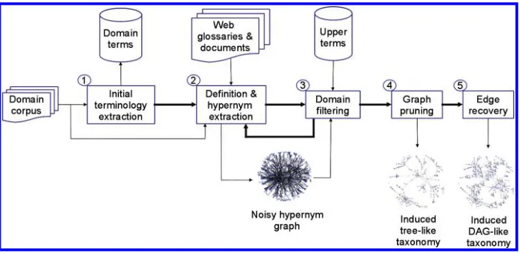
The OntoLearn Reloaded taxonomy learning workflow.
“automatically building” a taxonomy needs also to be demonstrated on new domains for which no a priori knowledge is available, however. In an unknown domain, tax-onomy induction requires the solution of several further problems, such as identifying domain-appropriate concepts, extracting appropriate hypernym relations, and detect-ing lexical ambiguity, whereas some of these problems can be ignored when evaluatdetect-ing against a gold standard (we will return to this issue in detail in Section 4). In fact, the predecessor of OntoLearn Reloaded, that is, OntoLearn (Navigli and Velardi 2004), suffers from a similar problem, in that it relies on the WordNet taxonomy to establish paradigmatic connections between concepts.
3. The Taxonomy Learning Workflow
OntoLearn Reloaded starts from an initially empty directed graph and a corpus for the domain of interest (e.g., an archive of artificial intelligence papers). We also assume that a small set of upper terms (entity, abstraction, etc.), which we take as the end points of our algorithm, has been manually defined (e.g., from a general purpose taxon-omy like WordNet) or is available for the domain.4Our taxonomy-learning workflow, summarized in Figure 1, consists of five steps:
1. Initial Terminology Extraction (Section 3.1):The first step applies a term extraction algorithm to the input domain corpus in order to produce an initial domain terminology as output.
2. Definition & Hypernym Extraction (Section 3.2):Candidate definition sentences are then sought for the extracted domain terminology. For each termt, adomain-independent classifieris used to select well-formed definitions from the candidate sentences and extract the corresponding hypernyms oft.
3. Domain Filtering (Section 3.3):A domain filtering technique is applied to filter out those definitions that do not pertain to the domain of interest. The resulting domain definitions are used to populate the directed graph with hypernymy relations connectingtto the extracted hypernymh. Steps (2) and (3) are then iterated on the newly acquired hypernyms, until a termination condition occurs.
4. Graph Pruning (Section 3.4):As a result of the iterative phase we obtain a dense hypernym graph that potentially contains cycles and multiple hypernyms for most nodes. In this step we combine a novel weighting strategy with the Chu-Liu/Edmonds algorithm (Chu and Liu 1965; Edmonds 1967) to produce an optimal branching (i.e., a tree-like taxonomy) of the initial noisy graph.
5. Edge Recovery (Section 3.5):Finally, we optionally apply a recovery strategy to reattach some of the hypernym edges deleted during the previous step, so as to produce a full-fledged taxonomy in the form of a DAG.
We now describe in full detail the five steps of OntoLearn Reloaded.5
3.1 Initial Terminology Extraction
Domain terms are the building blocks of a taxonomy. Even though in many cases an initial domain terminology is available, new terms emerge continuously, especially in novel or scientific domains. Therefore, in this work we aim at fully automatizing the taxonomy induction process. Thus, we start from a text corpus for the domain of interest and extract domain terms from the corpus by means of a terminology extraction algorithm. For this we use our term extraction tool, TermExtractor,6 that implements measures of domain consensus and relevance to harvest the most relevant terms for the domain from the input corpus.7 As a result, an initial domain terminol-ogyT(0) is produced that includes both single- and multi-word expressions (such as, respectively, graphand flow network). We add one node to our initially empty graph Gnoisy=(Vnoisy,Enoisy) for each term inT(0)—that is, we setVnoisy:=T(0)andEnoisy:=∅.
In Table 1 we show an excerpt of our ARTIFICIAL INTELLIGENCE and FINANCE
terminologies (cf. Section 4 for more details). Note that our initial set of domain terms (and, consequently, nodes) will be enriched with the new hypernyms acquired during the subsequent iterative phase, described in the next section.
3.2 Definition and Hypernym Extraction
The aim of our taxonomy induction algorithm is to learn a hypernym graph by means of several iterations, starting fromT(0)and stopping at very general termsU, that we take as the end point of our algorithm. The upper terms are chosen from WordNet topmost
5 A video of the first four steps of OntoLearn Reloaded is available at http://www.youtube.com/watch?v=-k3cOEoI Dk.
6http://lcl.uniroma1.it/termextractor.
Table 1
An excerpt of the terminology extracted for the ARTIFICIALINTELLIGENCEand FINANCE domains.
ARTIFICIALINTELLIGENCE
acyclic graph parallel corpus flow network
adjacency matrix parse tree pattern matching
artificial intelligence partitioned semantic network pagerank
tree data structure pathfinder taxonomic hierarchy
FINANCE
investor shareholder open economy
bid-ask spread profit maximization speculation
long term debt shadow price risk management
optimal financing policy ratings profit margin
synsets. In other words,U contains all the terms in the selected topmost synsets. In Table 2 we show representative synonyms of the upper-level synsets that we used for the ARTIFICIAL INTELLIGENCE and FINANCEdomains. Seeing that we use high-level concepts, the setUcan be considered domain-independent. Other choices are of course possible, especially if an upper ontology for a given domain is already available.
For each termt∈T(i)(initially,i=0), we first check whethertis an upper term (i.e., t∈U). If it is, we just skip it (because we do not aim at extending the taxonomy beyond an upper term). Otherwise, definition sentences are sought fortin the domain corpus and in a portion of the Web. To do so we use Word-Class Lattices (WCLs) (Navigli and Velardi 2010, introduced hereafter), which is a domain-independent machine-learned classifier that identifies definition sentences for the given term t, together with the corresponding hypernym (i.e., lexical generalization) in each sentence.
For each term in our setT(i), we then automatically extract definition candidates from the domain corpus, Web documents, and Web glossaries, by harvesting all the sentences that containt. To obtain on-line glossaries we use a Web glossary extraction system (Velardi, Navigli, and D’Amadio 2008). Definitions can also be obtained via a lightweight bootstrapping process (De Benedictis, Faralli, Navigli 2013).
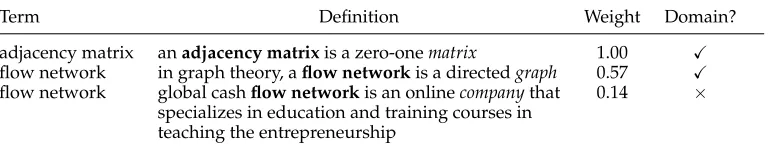
[image:7.486.56.420.575.666.2]Finally, we apply WCLs and collect all those sentences that are classified as defini-tional. We show some terms with their definitions in Table 3 (first and second column, respectively). The extracted hypernym is shown in italics.
Table 2
The set of upper concepts used in OntoLearn Reloaded for AI and FINANCE(only representative synonyms from the corresponding WordNet synsets are shown).
ability#n#1 abstraction#n#6 act#n#2 code#n#2
communication#n#2 concept#n#1 data#n#1 device#n#1 discipline#n#1 entity#n#1 event#n#1 expression#n#6
Table 3
Some definitions for the ARTIFICIALINTELLIGENCEdomain (defined term in bold, extracted hypernym in italics).
Term Definition Weight Domain?
adjacency matrix anadjacency matrixis a zero-onematrix 1.00 flow network in graph theory, aflow networkis a directedgraph 0.57 flow network global cashflow networkis an onlinecompanythat
specializes in education and training courses in teaching the entrepreneurship
0.14 ×
Table 4
Example definitions (defined terms are marked in bold face, their hypernyms in italics).
[In arts, achiaroscuro]DF[is]VF[a monochromepicture]GF.
[In mathematics, agraph]DF[is]VF[adata structure]GF[that consists of . . . ]REST. [In computer science, apixel]DF[is]VF[adot]GF[that is part of a computer image]REST. [Myrtales]DF[are an order of]VF[flowering plants]GF[placed as a basal group . . . ]REST.
3.2.1 Word-Class Lattices.We now describe our WCL algorithm for the classification of definitional sentences and hypernym extraction. Our model is based on a formal notion of textual definition. Specifically, we assume a definition contains the following fields (Storrer and Wellinghoff 2006):
r
The DEFINIENDUMfield (DF): this part of the definition includes the definiendum(that is, the word being defined) and its modifiers (e.g., “In computer science, apixel”);r
The DEFINITORfield (VF): which includes the verb phrase used to introduce the definition (e.g., “is”);r
The DEFINIENSfield (GF): which includes thegenus phrase(usually including the hypernym, e.g., “adot”);r
The RESTfield (RF): which includes additional clauses that further specify thedifferentiaof the definiendum with respect to its genus (e.g., “that is part of a computer image”).To train our definition extraction algorithm, a data set of textual definitions was manually annotated with these fields, as shown in Table 4.8 Furthermore, the single-or multi-wsingle-ord expression denoting the hypernym was also tagged. In Table 4, fsingle-or each sentence thedefiniendumand its hypernym are marked in bold and italics, respectively. Unlike other work in the literature dealing with definition extraction (Hovy et al. 2003; Fahmi and Bouma 2006; Westerhout 2009; Zhang and Jiang 2009), we covered not only a variety of definition styles in our training set, in addition to the classicX is a Ypattern, but also a variety of domains. Therefore, our WCL algorithm requires no re-training when changing the application domain, as experimentally demonstrated by Navigli and Velardi (2010). Table 5 shows some non-trivial patterns for the VF field.
Table 5
Some nontrivial patterns for the VF field.
is a term used to describe is a specialized form of
is the genus of was coined to describe
is a term that refers to a kind of is a special class of
can denote is the extension of the concept of
is commonly used to refer to is defined both as
Starting from the training set, the WCL algorithm learns generalized definitional models as detailed hereafter.
Generalized sentences.First, training and test sentences are part-of-speech tagged with the TreeTagger system, a part-of-speech tagger available for many languages (Schmid 1995). The first step in obtaining a definitional pattern is word generalization. Depending on its frequency we define a word class as either a word itself or its part of speech. Formally, letT be the set of training sentences. We first determine the setFof words inT whose frequency is above a thresholdθ(e.g.,the,a,an,of). In our training sentences, we replace the defined term with the tokenTARGET (note thatTARGET ∈F).
Given a new sentences=t1,t2,. . .,tn, wheretiis thei-th token ofs, we generalize
its wordstito word classestias follows:
ti =
ti ifti∈F
POS(ti) otherwise
that is, a wordti is left unchanged if it occurs frequently in the training corpus (i.e.,
ti∈F); otherwise it is replaced with its part of speech (POS(ti)). As a result we obtain a
generalized sentences. For instance, given the first sentence in Table 4, we obtain the corresponding generalized sentence: “In NNS, aTARGET is a JJ NN,” where NN and JJ indicate the noun and adjective classes, respectively. Generalized sentences are dou-bly beneficial: First, they help reduce the annotation burden, in that many differently lexicalized sentences can be caught by a single generalized sentence; second, thanks to their reduction of the definition variability, they allow for a higher-recall definition model.
Star patterns.LetT again be the set of training sentences. In this step we associate a star patternσ(s) with each sentences∈T. To do so, lets∈T be a sentence such that
s=t1,t2,. . .,tn, whereti is itsi-th token. Given the setFof most frequent words inT,
the star patternσ(s) associated withsis obtained by replacing with * all the tokensti∈F,
that is, all the tokens that are non-frequent words. For instance, given the sentence “In arts, a chiaroscuro is a monochrome picture,” the corresponding star pattern is “In *, a TARGET is a *,” whereTARGET is the defined term.
Sentence clustering.We then cluster the sentences in our training setT on the basis of their star pattern. Formally, letΣ =(σ1,. . .,σm) be the set of star patterns associated
with the sentences inT. We create a clusteringC=(C1,. . .,Cm) such thatCi={s∈T :
σ(s)=σi}, that is,Cicontains all the sentences whose star pattern isσi.
sentences whose degree of variability is generally much lower than for any pair of sentences inT belonging to two different clusters.
Word-class lattice construction.The final step consists of the construction of a WCL for each sentence cluster, using the corresponding generalized sentences. Given such a clusterCi∈C, we apply a greedy algorithm that iteratively constructs the WCL.
LetCi={s1,s2,. . .,s|Ci|}and consider its first sentences1=t1,t2,. . .,tn. Initially, we
create a directed graphG=(V,E) such thatV={t1,. . .,tn}andE={(t1,t2), (t2,t3),. . ., (tn−1,tn)}. Next, for eachj=2,. . .,|Ci|, we determine the alignment between sentencesj
and each sentencesk∈Cisuch thatk<jaccording to the following dynamic
program-ming formulation (Cormen, Leiserson, and Rivest 1990, pages 314–319):
Ma,b=max{Ma−1,b−1+Sa,b,Ma,b−1,Ma−1,b}, (1)
wherea∈ {0,. . .,|sk|}andb∈ {0,. . .,|sj|},Sa,b is a score of the matching between the
a-th token ofskand theb-th token ofsj, andM0,0,M0,bandMa,0are initially set to 0 for all values ofaandb.
The matching score Sa,b is calculated on the generalized sentences skandsj as
follows:
Sa,b=
1 iftk,a=tj,b 0 otherwise
wheretk,aandtj,bare thea-th andb-th tokens ofskandsj, respectively. In other words, the matching score equals 1 if thea-th and theb-th tokens of the two generalized sentences have the same word class.
Finally, the alignment score betweenskandsjis given byM|sk|,|sj|, which calculates
the minimal number of misalignments between the two token sequences. We repeat this calculation for each sentencesk(k=1,. . .,j−1) and choose the one that maximizes its
alignment score withsj. We then use the best alignment to addsjto the graphG: We add
to the set of nodesVthe tokens ofsjfor which there is no alignment toskand we add to Ethe edges (t1,t2),. . ., (t|s
j|−1,t
|sj|).
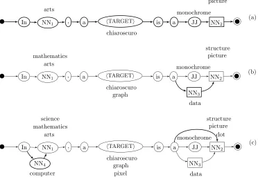
Example. Consider the first three definitions in Table 4. Their star pattern is “In *, a TARGET is a *.” The corresponding WCL is built as follows: The first part-of-speech tagged sentence, “In/IN arts/NN , a/DT TARGET /NN is/VBZ a/DT monochrome/JJpicture/NN,” is considered. The corresponding generalized sentence is “In NN1, aTARGET is a JJNN2.” The initially empty graph is thus populated with one node for each word class and one edge for each pair of consecutive tokens, as shown in Figure 2a. Note that we use a rectangle to denote the hypernym token NN2 . We also add
to the graph a start node
r
and an end noder
, and connect them to the corresponding initial and final sentence tokens. Next, the second sentence, “In mathematics, a graph is a data structure that consists of...,” is aligned to the first sentence. The alignment is perfect, apart from the NN3 node corresponding to “data.” The node is added tothe graph together with the edges “a”→ NN3 and NN3 →NN2 (Figure 2b, node and
Figure 2
The Word-Class Lattice construction steps on the first three sentences in Table 4. We show in bold the nodes and edges added to the lattice graph as a result of each sentence alignment step. The support of each word class is reported beside the corresponding node.
edges are added that connect node “In” to NN4and NN4to NN1. Figure 2c shows the resulting lattice.
Variants of the WCL model.So far we have assumed that our WCL model learns lattices from the training sentences in their entirety (we call this model WCL-1). We also consid-ered a second model that, given a star pattern, learns three separate WCLs, one for each of the three main fields of the definition, namely: definiendum (DF), definitor (VF), and definiens (GF). We refer to this latter model as WCL-3. Note that our model does not take into account the RESTfield, so this fragment of the training sentences is discarded. The reason for introducing the WCL-3 model is that, whereas definitional patterns are highly variable, DF, VF, and GF individually exhibit a lower variability, thus WCL-3 improves the generalization power.
Once the learning process is over, a set of WCLs is produced. Given a test sentence s, the classification phase for the WCL-1 model consists of determining whether there exists a lattice that matchess. In the case of WCL-3, we consider any combination of definiendum, definitor, and definiens lattices. Given that different combinations might match, for each combination of three WCLs we calculate a confidence score as follows:
score(s,lDF,lVF,lGF)=coverage·log2(support+1) (2)
third lattice, and support is the total number of sentences in the corresponding star pattern.
WCL-3 selects, if any, the combination of the three WCLs that best fits the sentence in terms of coverage and support from the training set. In fact, choosing the most appropriate combination of lattices impacts the performance of hypernym extraction. Given its higher performance (Navigli and Velardi 2010), in OntoLearn Reloaded we use WCL-3 for definition classification and hypernym extraction.
3.3 Domain Filtering and Creation of the Hypernym Graph
The WCLs described in the previous section are used to identify definitional sentences and harvest hypernyms for the terms obtained as a result of the terminology extraction phase. In this section we describe how to filter out non-domain definitions and create a dense hypernym graph for the domain of interest.
Given a term t, the common case is that several definitions are found for it (e.g., the flow network example provided at the beginning of this section). Many of these will not pertain to the domain of interest, however, especially if they are obtained from the Web or if they define ambiguous terms. For instance, in the COMPUTER
SCIENCE domain, the cash flow definition of flow network shown in Table 3 was not pertinent. To discard these non-domain sentences, we weight each definition candidate d(t) according to the domain terms that are contained therein using the following formula:
DomainWeight(d(t))= |Bd(t)∩D|
|Bd(t)| (3)
whereBd(t)is the bag of content words in the definition candidated(t) andDis given by the union of the initial terminologyT(0)and the set of single words of the terms in T(0) that can be found as nouns in WordNet. For example, given T(0) ={greedy algo-rithm,information retrieval,minimum spanning tree}, our domain terminologyD=T(0)∪ {algorithm,information,retrieval,tree}. According to Equation (3), the domain weight of a definition is normalized by the total number of content words in the definition, so as to penalize longer definitions. Domain filtering is performed by keeping only those definitionsd(t) whoseDomainWeight(d(t))≥θ, whereθis an empirically tuned thresh-old.9In Table 3 (third column), we show some values calculated for the corresponding definitions (the fourth column reports a check mark if the domain weight is above the threshold, an×otherwise). Domain filtering performs some implicit form of Word Sense Disambiguation (Navigli 2009), as it aims at discarding senses of hypernyms which do not pertain to the domain.
LetHtbe the set of hypernyms extracted with WCLs from the definitions of termt
which survived this filtering phase. For eacht∈T(i), we addHtto our graphGnoisy=
(Vnoisy,Enoisy), that is, we set Vnoisy:=Vnoisy∪Ht. For each t, we also add a directed
edge (h,t)10for each hypernymh∈Ht, that is, we setEnoisy:=Enoisy∪ {(h,t)}. As a result
9 Empirically set to 0.38, as a result of tuning on several data sets of manually annotated definitions in different domains.
of this step, the graph contains our domain terms and their hypernyms obtained from domain-filtered definitions. We now set:
T(i+1):=
t∈T(i)
Ht \ i
j=1
T(j) (4)
that is, the new set of termsT(i+1)is given by the hypernyms of the current set of terms T(i) excluding those terms that were already processed during previous iterations of the algorithm. Next, we move to iterationi+1 and repeat the last two steps, namely, we perform definition/hypernym extraction and domain filtering onT(i+1). As a result of subsequent iterations, the initially empty graph is increasingly populated with new nodes (i.e., domain terms) and edges (i.e., hypernymy relations).
After a given number of iterations K, we obtain a dense hypernym graph Gnoisy
that potentially contains more than one connected component. Finally, we connect all the upper term nodes inGnoisyto a single top node . As a result of this connecting
step, only one connected component of the noisy hypernym graph—which we call the backbone component—will contain an upper taxonomy consisting of upper terms inU.
The resulting graphGnoisypotentially contains cycles and multiple hypernyms for
the vast majority of nodes. In order to eliminate noise and obtain a full-fledged taxon-omy, we perform a step of graph pruning, as described in the next section.
3.4 Graph Pruning
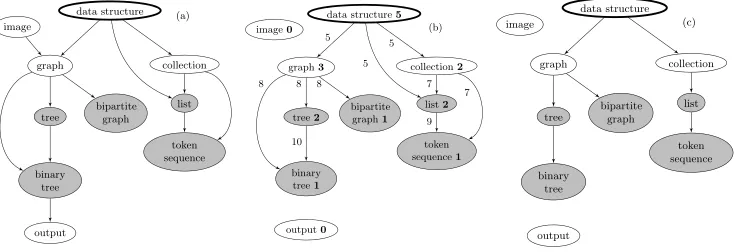
At the end of the iterative hypernym harvesting phase, described in Sections 3.2 and 3.3, the result is a highly dense, potentially disconnected, hypernymy graph (see Section 4 for statistics concerning the experiments that we performed). Wrong nodes and edges might stem from errors in any of the definition/hypernym extraction and domain filter-ing steps. Furthermore, for each node, multiple “good” hypernyms can be harvested. Rather than using heuristic rules, we devised a novel graph pruning algorithm, based on the Chu-Liu/Edmonds optimal branching algorithm (Chu and Liu 1965; Edmonds 1967), that exploits the topological graph properties to produce a full-fledged taxonomy. The algorithm consists of four phases (i.e., graph trimming, edge weighting, optimal branching, and pruning recovery) that we describe hereafter with the help of the noisy graph in Figure 3a, whose grey nodes belong to the initial terminologyT(0)and whose bold node is the only upper term.
3.4.1 Graph Trimming.We first perform two trimming steps. First, we disconnect “false” roots, i.e., nodes which are not in the set of upper terms and with no incoming edges (e.g.,imagein Figure 3a). Second, we disconnect “false” leaves, namely, leaf nodes which are not in the initial terminology and with no outgoing edges (e.g.,outputin Figure 3a). We show the disconnected components in Figure 3b.
3.4.2 Edge Weighting.Next, we weight the edges in our noisy graphGnoisy. A policy based
only on graph connectivity (e.g., in-degree or betweenness, see Newman [2010] for a complete survey) is not sufficient for taxonomy learning.11Consider again the graph in
Figure 3
A noisy graph excerpt (a), its trimmed version (b), and the final taxonomy resulting from pruning (c).
Figure 3: In choosing the best hypernym for the termtoken sequence, a connectivity-based measure might selectcollectionrather thanlist, because the former reaches more nodes. In taxonomy learning, however, longer hypernymy paths should be preferred (e.g.,data structure→collection→list→token sequenceis better thandata structure→collection→ token sequence).
We thus developed a novel weighting policy aimed at finding the best trade-off between path length and the connectivity of traversed nodes. It consists of three steps:
i) Weight each nodevby the number of nodes belonging to the initial terminology that can be reached fromv(potentially includingvitself).12 Letw(v) denote the weight ofv(e.g., in Figure 3b, nodecollectionreaches listandtoken sequence, thusw(collection)=2, whereasw(graph)=3). All weights are shown in the corresponding nodes in Figure 3b.
ii) For each nodev, consider all the paths from an upper rootrtov. LetΓ(r,v) be the set of such paths. Each pathp∈Γ(r,v) is weighted by the cumulative weight of the nodes in the path, namely:
ω(p)=
v∈p
w(v) (5)
iii) Assign the following weight to each incoming edge (h,v) ofv(i.e.,his one of the direct hypernyms ofv):
w(h,v)=max
r∈U p∈maxΓ(r,h)ω(p) (6) This formula assigns to edge (h,v) the valueω(p) of the highest-weighting pathpfromhto any upper root∈U. For example, in Figure 3b,w(list)=2, w(collection)=2,w(data structure)=5. Therefore, the set of pathsΓ(data structure,list) ={data structure→list,data structure→collection→list}, whose weights are 7 (w(data structure) +w(list)) and 9 (w(data structure) + w(collection) +w(list)), respectively. Hence, according to Formula 6,w(list, token sequence)=9. We show all edge weights in Figure 3b.
3.4.3 Optimal Branching. Next, our goal is to move from a noisy graph to a tree-like taxonomy on the basis of our edge weighting strategy. A maximum spanning tree algorithm cannot be applied, however, because our graph is directed. Instead, we need to find an optimal branching, that is, a rooted tree with an orientation such that every node but the root has in-degree 1, and whose overall weight is maximum. To this end, we first apply a pre-processing step: For each (weakly) connected component in the noisy graph, we consider a number of cases, aimed at identifying a single “reasonable” root node to enable the optimal branching to be calculated. LetRbe the set of candidate roots, that is, nodes with no incoming edges. We perform the following steps:
i) If|R|=1 then we select the only candidate as root.
ii) Else if|R|>1, if an upper term is inR, we select it as root, else we choose the rootr∈Rwith the highest weightwaccording to the weighting strategy described in Section 3.4.2. We also disconnect all the unselected roots, that is, those inR\ {r}.
iii) Else (i.e., if|R|=0), we proceed as for step (ii), but we search candidates within the entire connected component and select the highest weighting node. In contrast to step (ii), we remove all the edges incoming to the selected node.
This procedure guarantees not only the selection but also the existence of a single root node for each component, from which the optimal branching algorithm can start. We then apply the Chu-Liu/Edmonds algorithm (Chu and Liu 1965; Edmonds 1967) to each componentGi=(Vi,Ei) of our directed weighted graphGnoisyin order to find an
optimal branching. The algorithm consists of two phases: acontraction phase and an expansionphase. The contraction phase is as follows:
1. For each node which is not a root, we select the entering edge with the highest weight. LetSbe the set of such|Vi| −1 edges;
2. If no cycles are formed inS, go to the expansion phase. Otherwise, continue;
3. Given a cycle inS, contract the nodes in the cycle into a pseudo-nodek, and modify the weight of each edge entering any nodevin the cycle from some nodehoutside the cycle, according to the following equation:
w(h,k)=w(h,v)+(w(x(v),v)−minv(w(x(v),v))) (7)
wherex(v) is the predecessor ofvin the cycle andw(x(v),v) is the weight of the edge in the cycle which entersv;
4. Select the edge entering the cycle which has the highest modified weight and replace the edge which enters the same real node inSby the new selected edge;
5. Go to step 2 with the contracted graph.
Gi (i.e., thei-th component ofGnoisy). During the expansion phase, pseudo-nodes are
replaced with the original cycles. To break the cycle, we select the real nodevinto which the edge selected in step 4 enters, and remove the edge entering v belonging to the cycle. Finally, the weights on the edges are restored. For example, consider the cycle in Figure 4a. Nodes pagerank, map, andrank are contracted into a pseudo-node, and the edges entering the cycle from outside are re-weighted according to Equation (7). According to the modified weights (Figure 4b), the selected edge, that is, (table,map), is the one with weightw=13. During the expansion phase, the edge (pagerank,map) is eliminated, thus breaking the cycle (Figure 4c).
The tree-like taxonomy resulting from the application of the Chu-Liu/Edmonds algorithm to our example in Figure 3b is shown in Figure 3c.
3.4.4 Pruning Recovery. The weighted directed graph Gnoisy input to the Chu-Liu/
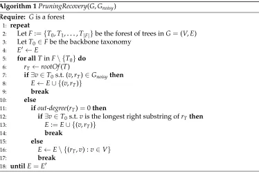
Edmonds algorithm might contain many (weakly) connected components. In this case, an optimal branching is found for each component, resulting in a forest of taxonomy trees. Although some of these components are actually noisy, others provide an impor-tant contribution to the final tree-like taxonomy. The objective of this phase is to recover from excessive pruning, and re-attach some of the components that were disconnected during the optimal branching step. Recall from Section 3.3 that, by construction, we have only one backbone component, that is, a component which includes an upper tax-onomy. Our aim is thus to re-attach meaningful components to the backbone taxtax-onomy. To this end, we apply Algorithm 1. The algorithm iteratively merges non-backbone trees to the backbone taxonomy treeT0in three main steps:
r
Semantic reconnection step(lines 7–9 in Algorithm 1): In this step we reuse a previously removed “noisy” edge, if one is available, to reattach a non-backbone component to the backbone. Given a root noderTi of anon-backbone treeTi(i>0), if an edge (v,rTi) existed in the noisy graph
Gnoisy(i.e., the one obtained before the optimal branching phase), with
[image:16.486.51.418.465.618.2]v∈T0, then we connect the entire treeTitoT0by means of this edge.
Figure 4
Algorithm 1PruningRecovery(G,Gnoisy)
Require: Gis a forest
1: repeat
2: LetF:={T0,T1,. . .,T|F|}be the forest of trees inG=(V,E)
3: LetT0∈Fbe the backbone taxonomy
4: E←E
5: for allTinF\ {T0}do
6: rT←rootOf(T)
7: if∃v∈T0s.t. (v,rT)∈Gnoisythen
8: E←E∪ {(v,rT)}
9: break
10: else
11: ifout-degree(rT)=0then
12: if∃v∈T0s.t.vis the longest right substring ofrTthen
13: E:=E∪ {(v,rT)}
14: break
15: else
16: E←E\ {(rT,v) :v∈V}
17: break
18: untilE=E
r
Reconnection step by lexical inclusion(lines 11–14): Otherwise, ifTiis a singleton (the out-degree ofrTi is 0) and there exists a nodev∈T0suchthatvis the longest right substring ofrTiby lexical inclusion,
13we connect Tito the backbone treeT0by means of the edge (v,rTi).
r
Decomposition step(lines 15–17): Otherwise, if the componentTiis not a singleton (i.e., if the out-degree of the root noderTiis>0) we disconnectrTifromTi. At first glance, it might seem counterintuitive to remove edges
during pruning recovery. Reconnecting by lexical inclusion within a domain has already been shown to perform well in the literature (Vossen 2001; Navigli and Velardi 2004), but we want to prevent any cascading errors on the descendants of the root node, and at the same time free up other pre-existing “noisy” edges incident to the descendants.
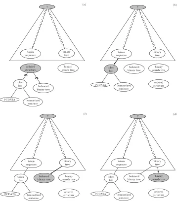
These three steps are iterated on the newly created components, until no change is made to the graph (line 18). As a result of our pruning recovery phase we return the enriched backbone taxonomy. We show in Figure 5 an example of pruning recovery that starts from a forest of three components (including the backbone taxonomy tree on top, Figure 5a). The application of the algorithm leads to the disconnection of a tree root, that is,ordered structure(Figure 5a, lines 15–17 of Algorithm 1), the linking of the trees rooted attoken listandbinary search treeto nodes in the backbone taxonomy (Figures 5b and 5d, lines 7–9), and the linking ofbalanced binary treetobinary treethanks to lexical inclusion (Figure 5c, lines 11–14 of the algorithm).
13 Similarly to our original OntoLearn approach (Navigli and Velardi 2004), we define a node’s string v=wnwn−1. . .w2w1to be lexically included in that of a nodev=wmwm−1. . .w2w1ifm>nand
[image:17.486.56.430.62.313.2]Figure 5
An example starting with three components, including the backbone taxonomy tree on the top and two other trees on the bottom (a). As a result of pruning recovery, we disconnectordered structure(a); we connecttoken sequencetotoken listby means of a “noisy” edge (b); we connect
binary treetobalanced binary treeby lexical inclusion (c); and finallybinary treetobinary search treeby means of another “noisy” edge (d).
3.5 Edge Recovery
procedureandtraining algorithm, so two hypernym edges should correctly be incident to thebackpropagationnode.
We start from our backbone taxonomy T0 obtained after the pruning recovery phase described in Section 3.4.4. In order to obtain a DAG-like taxonomy we apply the following step: for each “noisy” edge (v,v)∈Enoisysuch thatv,vare nodes inT0 but the edge (v,v) does not belong to the tree, we add (v,v) toT0if:
i) it does not create a cycle inT0;
ii) the absolute difference between the length of the shortest path fromvto the rootrT0and that of the shortest path fromv
tor
T0is within an interval
[m,M]. The aim of this constraint is to maintain a balance between the height of a concept in the tree-like taxonomy and that of the hypernym considered for addition. In other words, we want to avoid the connection of an overly abstract concept with an overly specific one.
In Section 4, we experiment with three versions of our OntoLearn Reloaded algo-rithm, namely: one version that does not perform edge recovery (i.e., which learns a tree-like taxonomy [TREE], and two versions that apply edge recovery (i.e., which learn a DAG) with different intervals for constraint (ii) above (DAG[1, 3] andDAG[0, 99]; note that the latter version virtually removes constraint (ii)). Examples of recovered edges will be presented and discussed in the evaluation section.
3.6 Complexity
We now perform a complexity analysis of the main steps of OntoLearn Reloaded. Given the large number of steps and variables involved we provide a separate discussion of the main costs for each individual step, and we omit details about commonly used data structures for access and storage, unless otherwise specified. LetGnoisy=(Vnoisy,Enoisy)
be our noisy graph, and letn=|Vnoisy|andm=|Enoisy|.
1. Terminology extraction:Assuming a part-of-speech tagged corpus as input, the cost of extracting candidate terms by scanning the corpus with a maximum-size window is in the order of the word size of the input corpus. Thus, the application of statistical measures to our set of candidate terms has a computational cost that is on the order of the square of the number of term candidates (i.e., the cost of calculating statistics for each pair of terms).
2. Definition and hypernym extraction:In the second step, we first retrieve candidate definitions from the input corpus, which costs on the order of the corpus size.14Each application of a WCL classifier to an input candidate sentencescontaining a termtcosts on the order of the word length of the sentence, and we have a constant number of such classifiers. So the cost of this step is given by the sum of the lengths of the candidate sentences in the corpus, which is lower than the word size of the corpus.
3. Domain filtering and creation of the graph:The cost of domain filtering for a single definition is in the order of its word length, so the running time of domain filtering is in the order of the sum of the word size of the acquired definitions. As for the hypernym graph creation, using an adjacency-list representation of the graphGnoisy, the dynamic addition of a
newly acquired hypernymy edge costsO(n), an operation which has to be repeated for each (hypernymy, term) pair.
4. Graph pruning, consisting of the following steps:
r
Graph trimming:This step requiresO(n) time in order to identify false leaves and false roots by iterating over the entire set of nodes.r
Edge weighting:i) We perform a DFS (O(n+m)) to weight all thenodes in the graph; ii) we collect all paths from upper roots to any given node, totalizingO(n!) paths in the worst case (i.e., in a complete graph). In real domains, however, the computational cost of this step will be much lower. In fact, over our six domains, the average number of paths per node ranges from 4.3 (n= 2107, ANIMALS) to 3175.1 (n= 2616, FINANCEdomain): In the latter, worst case, in practice, the number of paths is in the order ofn, thus the cost of this step, performed for each node, can be estimated by O(n2) running time; iii) assigning maximum weights to edges costs O(m) if in the previous step we keep track of the maximum value of paths ending in each nodeh(see Equation (6)).
r
Optimal branching:Identifying the connected components of our graph costsO(n+m) time, identifying root candidates and selecting one root per component costsO(n), and finally applying the Chu-Liu/Edmonds algorithm costsO(m·log2n) for sparse graphs,O(n2) for dense ones, using Tarjan’s implementation (Tarjan 1977).5. Pruning recovery:In the worst case,miterations of Algorithm 1 will be performed, each costingO(n) time, thus having a total worst-case cost of O(mn).
6. Edge recovery:For each pair of nodes inT0we perform i) the
identification of cycles (O(n+m)) and ii) the calculation of the shortest paths to the root (O(n+m)). By precomputing the shortest path for each node, the cost of this step isO(n(n+m)) time.
Therefore, in practice, the computational complexity of OntoLearn Reloaded is polynomial in the main variables of the problem, namely, the number of words in the corpus and nodes in the noisy graph.
4. Evaluation
the quality of a taxonomy. These include Brank, Mladenic, and Grobelnik (2006) and Maedche, Pekar, and Staab (2002):
a) automatic evaluation against a gold standard;
b) manual evaluation performed by domain experts;
c) structural evaluation of the taxonomy;
d) application-driven evaluation, in which a taxonomy is assessed on the basis of the improvement its use generates within an application.
Other quality indicators have been analyzed in the literature, such as accuracy, completeness, consistency (V ¨olker et al. 2008), and more theoretical features (Guarino and Welty 2002) like essentiality, rigidity, and unity. Methods (a) and (b) are by far the most popular ones. In this section, we will discuss in some detail the pros and cons of these two approaches.
Gold standard evaluation.The most popular approach for the evaluation of lexicalized taxonomies (adopted, e.g., in Snow, Jurafsky, and Ng 2006; Yang and Callan 2009; and Kozareva and Hovy 2010) is to attempt to reconstruct an existing gold standard (Maedche, Pekar, and Staab 2002), such as WordNet or the Open Directory Project. This method is applicable when the set of taxonomy concepts are given, and the evaluation task is restricted to measuring the ability to reproduce hypernymy links between concept pairs. The evaluation is far more complex when learning a specialized taxonomy entirely from scratch, that is, when both terms and relations are unknown. In reference taxonomies, even in the same domain, the granularity and cotopy15 of an abstract concept might vary according to the scope of the taxonomy and the expertise of the team who created it (Maedche, Pekar, and Staab 2002). For example, both the termschiaroscuroandcollageare classified underpicture, image, iconin WordNet, but in the Art & Architecture Thesaurus (AA&T)16 chiaroscurois categorized underperspective and shading techniques whereas collage is classified under image-making processes and techniques. As long as common-sense, non-specialist knowledge is considered, it is still feasible for an automated system to replicate an existing classification, because the Web will provide abundant evidence for it. For example, Kozareva and Hovy (2010, K&H hereafter) are very successful at reproducing the WordNet sub-taxonomy for
ANIMALS, because dozens of definitional patterns are found on the Web that classify,
for example, lionas a carnivorous feline mammal, or carnivorous, or feline. As we show later in this section, however, and as also suggested by the previous AA&T example, finding hypernymy patterns in more specialized domains is far more complex. Even in simpler domains, however, it is not clear how to evaluate the concepts and relations not found in the reference taxonomy. Concerning this issue, Zornitsa Kozareva comments that: “When we gave sets of terms to annotators and asked them to produce a taxonomy, people struggled with the domain terminology and produced quite messy organization. Therefore, we decided to go with WordNet and use it as a gold truth” (personal communication). Accordingly, K&H do not provide an evaluation of the nodes and relations other than those for which the ground truth is known. This is further clarified in a personal communication: “Currently we do not have a full list of all is-a outside
WordNet. [...] In the experiments, we work only with the terms present in WordNet [...] The evaluation is based only on the WordNet relations. However, the harvesting algorithm extracts much more. Currently, we do not know how to evaluate the Web taxonomization.”
To conclude, gold standard evaluation has some evident drawbacks:
r
When both concepts and relations are unknown, it is almost impossible to replicate a reference taxonomy accurately.r
In principle, concepts not in the reference taxonomy can be either wrong or correct; therefore the evaluation is in any case incomplete.Another issue in gold standard evaluation is the definition of an adequate evalu-ation metric. The most common measure used in the literature to compare a learned with a gold-standard taxonomy is the overlapping factor (Maedche, Pekar, and Staab 2002). Given the set of is-a relations in the two taxonomies, the overlapping factor simply computes the ratio between the intersection and union of these sets. Therefore the overlapping factor gives a useful global measure of the similarity between the two taxonomies. It provides no structural comparison, however: Errors or differences in grouping concepts in progressively more general classes are not evidenced by this measure.
Comparison against a gold standard has been analyzed in a more systematic way by Zavitsanos, Paliouras, and Vouros (2011) and Brank, Mladenic, and Grobelnik (2006). They propose two different strategies for escaping the “naming” problem that we have outlined. Zavitsanos, Paliouras, and Vouros (2011) propose transforming the ontology concepts and their properties into distributions over the term space of the source data from which the ontology has been learned. These distributions are used to compute pairwise concept similarity between gold standard and learned ontologies.
Brank, Mladenic, and Grobelnik (2006) exploit the analogy between ontology learn-ing and unsupervised clusterlearn-ing, and propose OntoRand, a modified version of the Rand Index (Rand 1971) for computing the similarity between ontologies. Morey and Agresti (1984) and Carpineto and Romano (2012), however, demonstrated a high de-pendency of the Rand Index (and consequently of OntoRand itself) upon the number of clusters, and Fowlkes and Mallows (1983) show that the Rand Index has the undesirable property of converging to 1 as the number of clusters increases, even in the unrealistic case of independent clusterings. These undesired outcomes have also been experienced by Brank, Mladenic, and Grobelnik (2006, page 5), who note that “the similarity of an ontology to the original one is still as high as 0.74 even if only the top three levels of the ontology have been kept.” Another problem with the OntoRand formula, as also remarked in Zavitsanos, Paliouras, and Vouros (2011), is the requirement of comparing ontologies with the same set of instances.
hypernymy relations “in isolation,” but must also provide a structural assessment aimed at identifying common phenomena and the overall quality of the taxonomic structure. Unfortunately, as already pointed out, manual evaluation is a hard task. Deciding whether or not a concept belongs to a given domain is more or less feasible for a domain expert, but assessing the quality of a hypernymy link is far more complex. On the other hand, asking a team of experts to blindly reconstruct a hierarchy, given a set of terms, may result in the “messy organization” reported by Zornitsa Kozareva. In contrast to previous approaches to taxonomy induction, OntoLearn Reloaded provides a natural solution to this problem, becauseis-alinks in the taxonomy are supported by one or more definition sentences from which the hypernymy relation was extracted. As shown later in this section, definitions proved to be a very helpful feature in supporting manual analysis, both for hypernym evaluation and structural assessment.
The rest of this section is organized as follows. We first describe the experimen-tal set-up (Section 4.1): OntoLearn Reloaded is applied to the task of acquiring six taxonomies, four of which attempt to replicate already existing gold standard sub-hierarchies in WordNet17 and in the MeSH medical ontology,18 and the other two are new taxonomies acquired from scratch. Next, we present a large-scale multi-faceted evaluation of OntoLearn Reloaded focused on three of the previously described eval-uation methods, namely: comparison against a gold standard, manual evaleval-uation, and structural evaluation. In Section 4.2 we introduce a novel measure for comparing an induced taxonomy against a gold standard one. Finally, Section 4.3 is dedicated to a manual evaluation of the six taxonomies.
4.1 Experimental Set-up
We now provide details on the set-up of our experiments.
4.1.1 Domains.We applied OntoLearn Reloaded to the task of acquiring six taxonomies: ANIMALS, VEHICLES, PLANTS, VIRUSES, ARTIFICIAL INTELLIGENCE, and FINANCE.
The first four taxonomies were used for comparison against three WordNet sub-hierarchies and the viruses sub-hierarchy of MeSH. The ANIMALS, VEHICLES, and
PLANTSdomains were selected to allow for comparison with K&H, who experimented on the same domains. The ARTIFICIAL INTELLIGENCEand FINANCEdomains are ex-amples of taxonomies truly built from the ground up, for which we provide a thorough manual evaluation. These domains were selected because they are large, interdisci-plinary, and continuously evolving fields, thus representing complex and specialized use cases.
4.1.2 Definition Harvesting.For each domain, definitions were sought in Wikipedia and in Web glossaries automatically obtained by means of a Web glossary extraction system (Velardi, Navigli, and D’Amadio 2008). For the ARTIFICIALINTELLIGENCEdomain we also used a collection consisting of the entire IJCAI proceedings from 1969 to 2011 and the ACL archive from 1979 to 2010. In what follows we refer to this collection as the “AI corpus.” For FINANCEwe used a combined corpus from the freely available collection ofJournal of Financial Economicsfrom 1995 to 2012 and fromReview Of Financefrom 1997 to 2012 for a total of 1,575 papers.
4.1.3 Terminology. For the ANIMALS, VEHICLES, PLANTS, and VIRUSES domains, the initial terminology was a fragment of the nodes of the reference taxonomies,19 sim-ilarly to, and to provide a fair comparison with, K&H. For the AI domain instead, the initial terminology was selected using our TermExtractor tool20 on the AI corpus. TermExtractor extracted over 5,000 terms from the AI corpus, ranked according to a combination of relevance indicators related to the (direct) document frequency, domain pertinence, lexical cohesion, and other indicators (Sclano and Velardi 2007). We manu-ally selected 2,218 terms from the initial set, with the aim of eliminating compounds like order of magnitude, empirical study,international journal, that are frequent but not domain relevant. For similar reasons a manual selection of terms was also applied to the terminology automatically extracted for the FINANCEdomain, obtaining 2,348 terms21 from those extracted by TermExtractor. An excerpt of extracted terms was provided in Table 1.
4.1.4 Upper Terms. Concerning the selection of upper terms U (cf. Section 3.2), again similarly to K&H, we used just one concept for each of the four domains focused upon: ANIMALS, VEHICLES, PLANTS, and VIRUSES. For the AI and FINANCEdomains, which are more general and complex, we selected from WordNet a core taxonomy of 32 upper conceptsU (resulting in 52 terms) that we used as a stopping criterion for our iterative definition/hypernym extraction and filtering procedure (cf. Section 3.2). The complete list of upper concepts was given in Table 2. WordNet upper concepts are general enough to fit most domains, and in fact we used the same setU for AI and FINANCE. Nothing, however, would have prevented us from using a domain-specific core ontology, such as the CRM-CIDOC core ontology for the domain of ART AND
ARCHITECTURE.22
4.1.5 Algorithm Versions and Structural Statistics.For each of the six domains we ran the three versions of our algorithm: without pruning recovery (TREE), with [1, 3] recovery (DAG[1, 3]), and with [0, 99] recovery (DAG[0, 99]), for a total of 18 experiments. We remind the reader that the purpose of the recovery process was to reattach some of the edges deleted during the optimal branching step (cf. Section 3.5).
Figure 6 shows an excerpt of the AI tree-like taxonomy under the nodedata structure. Notice that, even though the taxonomy looks good overall, there are still a few errors, such as “neuronis aneural network” and overspecializations like “networkis adigraph.” Figure 7 shows a sub-hierarchy of the FINANCEtree-like taxonomy under the concept value.
In Table 6 we give the structural details of the 18 taxonomies extracted for our six domains. In the table, edge and node compression refers to the number of surviving nodes and edges after the application of optimal branching and recovery steps to the noisy hypernymy graph. To clarify the table, consider the case of VIRUSES,DAG[1, 3]: we started with 281 initial terms, obtaining a noisy graph with 1,174 nodes and 1,859 edges. These were reduced to 297 nodes (i.e., 1,174–877) and 339 edges (i.e., 1,859–1,520) after pruning and recovery. Out of the 297 surviving nodes, 222 belonged to the initial
19 For ANIMALS, VEHICLES, and PLANTSwe used precisely the same seeds as K&H. 20http://lcl.uniroma1.it/termextractor.
21 These dimensions are quite reasonable for large technical domains: as an example,The Economist’s glossary of economic terms includes on the order of 500 terms (http://www.economist.com/ economics-a-to-z/).
Figure 6
An excerpt of the ARTIFICIALINTELLIGENCEtaxonomy.
terminology; therefore the coverage over the initial terms is 0.79 (222/281). This means that, for some of the initial terms, either no definitions were found, or the definition was rejected in some of the processing steps. The table also shows, as expected, that the term coverage is much higher for “common-sense” domains likeANIMALS,VEHICLES, and PLANTS, is still over 0.75 for VIRUSES and AI, and is a bit lower for FINANCE
(0.65). The maximum and average depth of the taxonomies appears to be quite variable, with VIRUSES and FINANCE at the two extremes. Finally, Table 6 reports in the last column the number of glosses (i.e., domain definitional sentences) obtained in each run. We would like to point out that providing textual glosses for the retrieved domain hypernyms is a novel feature that has been lacking in all previous approaches to ontology learning, and which can also provide key support to much-needed manual validation and enrichment of existing semantic networks (Navigli and Ponzetto 2012).
4.2 Evaluation Against a Gold Standard
Figure 7
An excerpt of the FINANCEtaxonomy.
(2006) idea of exploiting the analogy with unsupervised clustering but, rather than representing the two taxonomies as flat clusterings, we propose a measure that takes into account the hierarchical structure of the two analyzed taxonomies. Under this perspective, a taxonomy can be transformed into a hierarchical clustering by replacing each label of a non-leaf node (e.g.,perspective and shading techniques) with the transitive closure of its hyponyms (e.g.,cangiatismo, chiaroscuro, foreshortening, hatching).
4.2.1 Evaluation Model.Techniques for comparing clustering results have been surveyed in Wagner and Wagner (2007), although the only method for comparing hierarchical clusters, to the best of our knowledge, is that proposed by Fowlkes and Mallows (1983). Suppose that we have two hierarchical clusteringsH1andH2, with an identical set ofn objects. Letkbe the maximum depth of bothH1 andH2, andHjia cut of the hierarchy,
wherei∈ {0,. . .,k}is the cut level andj∈ {1, 2}selects the clustering of interest. Then, for each cuti, the two hierarchies can be seen as two flat clusteringsCi
1andCi2of then concepts. Wheni=0 the cut is a single cluster incorporating all the objects, and when i=kwe obtainnsingleton clusters. Now let:
r
n11be the number of object pairs that are in the same cluster in bothCi1 andCi2;
r
n00be the number of object pairs that are in different clusters in bothCi1 andCi2;
r
n10be the number of object pairs that are in the same cluster inCi1but not inCi