Modeling Regular Polysemy: A Study on the Semantic Classification of Catalan Adjectives

Semantic Classification of Catalan Adjectives

Gemma Boleda

Sabine Schulte im Walde

Toni Badia

Universitat Pompeu Fabra

We present a study on the automatic acquisition of semantic classes for Catalan adjectives from distributional and morphological information, with particular emphasis on polysemous adjec-tives. The aim is to distinguish and characterize broad classes, such as qualitative (gran‘big’) and relational (pulmonar‘pulmonary’) adjectives, as well as to identify polysemous adjectives such asecon `omic(‘economic|cheap’). We specifically aim at modeling regular polysemy, that is, types of sense alternations that are shared across lemmata. To date, both semantic classes for adjectives and regular polysemy have only been sparsely addressed in empirical computational linguistics.

Two main specific questions are tackled in this article. First, what is an adequate broad semantic classification for adjectives? We provide empirical support for the qualitative and relational classes as defined in theoretical work, and uncover one type of adjective that has not received enough attention, namely, the event-related class. Second, how is regular polysemy best modeled in computational terms? We present two models, and argue that the second one, which models regular polysemy in terms of simultaneous membership to multiple basic classes, is both theoretically and empirically more adequate than the first one, which attempts to identify independent polysemous classes. Our best classifier achieves 69.1% accuracy, against a 51% baseline.

1. Introduction

Adjectives are one of the most elusive parts of speech with respect to meaning. For example, it is very difficult to establish a broad classification of adjectives into semantic classes, analogous to a broad ontological classification of nouns (Raskin and Nirenburg

∗ Department of Translation and Language Sciences, Universitat Pompeu Fabra, Roc Boronat 138, 08018 Barcelona, Spain. E-mail:[email protected].

∗∗ E-mail:[email protected].

† E-mail:[email protected].

1998). This article tackles precisely this task, that is, thesemantic classification of adjectives, for Catalan. We aim at automatically inducing the semantic class for an adjective given its linguistic properties, as extracted from corpora and other resources.

The acquisition of semantic classes has been widely studied for verbs (Dorr and Jones 1996; McCarthy 2000; Korhonen, Krymolowski, and Marx 2003; Lapata and Brew 2004; Schulte im Walde 2006; Joanis, Stevenson, and James 2008) and, to a lesser extent, for nouns (Hindle 1990; Pereira, Tishby, and Lee 1993), but, with very few exceptions (Bohnet, Klatt, and Wanner 2002; Carvalho and Ranchhod 2003), not for adjectives. Fur-thermore, we cannot rely on a well-established classification for adjectives. The classes themselves are subject to experimentation. We will test two different classifications, analyzing the empirical properties of the classes and the problems in their definition.

Another significant challenge is posed by polysemy, or the fact that one and the same adjective can have multiple senses. Different senses may fall into different classes, such that it is no longer possible to identify one single semantic class per adjective. Moreover, many adjectives exhibit similar sense alternations, in a phenomenon known asregularorsystematic polysemy(Apresjan 1974; Copestake and Briscoe 1995). A special focus of the research presented, therefore, is on modeling regular polysemy. As an example of regular polysemy, take for instance the sense alternation for the adjective econ`omicexemplified in Example (1).Econ`omic, derived fromeconomia(‘economy’), can be translated as ‘economic, of the economy’, as in Example (1a), or as ‘cheap’, as in Example (1b). As we will see, each of these senses corresponds to a different semantic class in our classifications.

(1) a. recuperaci ´o recovery

econ `omica economy_SUFFIX ‘recovery of the economy’ b. pantalons

trousers

econ `omics economy_SUFFIX ‘cheap trousers’

Other adjectives exhibit similar sense alternations; for example, familiar (derived fromfam´ılia, ‘family’) andamor´os(derived fromamor, ‘love’), as shown in Example (2).

(2) a. reuni ´o meeting

familiar family_SUFFIX/

/ face

cara

family_SUFFIX

familiar

‘family meeting / familiar face’ b. problema

problem

amor ´os love_SUFFIX/

/ boy

noi

love_SUFFIX

amor ´os

‘love problem / lovely boy’

The first senses in Examples (1) and (2) have a transparent relation to the denotation of the deriving noun, as witnessed by the fact that they are translated as nouns in English (economy,family,love), whereas the other senses are translated as adjectives (cheap, famil-iar,lovely). For each of these adjectives, there is a relationship between the two senses, such that the sense alternations seem to correspond to a productive semantic process along the lines of Example (3) (Raskin and Nirenburg 1998, schema (43), page 173).

Because of the systematic semantic relationship between the two senses of these adjec-tives, they constitute an instance of regular polysemy. In this article, therefore, we not only address the acquisition of semantic classes, but also theacquisition of polysemy: Our goal is to determine, for a given adjective, whether it is monosemous or polysemous, and to which class(es) it belongs. Note that we are not dealing with individual sense alternations, as related work on sense induction does (Sch ¨utze 1998; McCarthy et al. 2004; Brody and Lapata 2009), but with sense alternationtypes, that systematically hold across different lemmata. Thus, the present research is at the crossroad between sense induction and lexical acquisition.

Regularities in sense alternations are pervasive in human languages, and they are probably favored by the properties of human cognition (Murphy 2002). Regular polysemy has been studied in theoretical linguistics (Apresjan 1974; Pustejovsky 1995) and in symbolic approaches to computational semantics (Copestake and Briscoe 1995). It has received little attention in empirical computational semantics, however. This is surprising, given the amount of work devoted to sense-related tasks such as Word Sense Disambiguation (WSD). In WSD (see Navigli [2009] for an overview) sense ambiguities are almost exclusively modeled for each individual lemma, despite the ensuing sparsity problems (Ando [2006] is an exception). Properly modeling regular polysemy, therefore, promises to improve computational semantic tasks such as WSD and sense discrimination.

This article has the goal of finding a computational model that responds to the theoretical and empirical properties of regular polysemy. In this direction, we test two alternative approaches. We first model polysemy in terms of independent classes to be separately acquired (e.g., an adjective with two sensesa_iand b_ibelongs to a class AB defined independently of classes A and B), and showthat this model is not adequate. A second approach, which posits that polysemous adjectives simultaneously belong to more than one class (e.g., an adjective with two sensesai andbibelongs to both class A and class B), is more successful. Our best classifier achieves 69.1% accuracy against a 51% baseline, which is satisfactory, considering that the estimated upper bound (human agreement) for this task is 68%. We discuss pros and cons of the two models described and ways to overcome their limitations.

In the following, we first review related work (Section 2) and linguistic aspects of adjective classification (Section 3), then present the two acquisition experiments (Sections 4 and 5), and finish with a general discussion (Section 6) and some conclusions and directions for future research (Section 7).

2. Related Work

used is not purely semantic, polysemy is not taken into account, and the evidence and techniques used are more limited than the ones used here.

Other research on adjectives within computational linguistics is oriented toward different goals than ours. Yallop, Korhonen, and Briscoe (2005) tackle syntactic, not semantic classification, akin to the acquisition of subcategorization frames for verbs. Another relevant line of research pursues WSD. Justeson and Katz (1995) and Chao and Dyer (2000) showed that adjectives are a very useful cue for disambiguating the sense of the nouns they modify. Adjective classes could be further exploited in WSD in at least two respects: (1) to establish an inventory of adjective senses (if polysemous instances are correctly detected; this is where sense induction and our own work fits in), and (2) to exploit class-based properties for the disambiguation, similar to related work on verb classes (Resnik 1993; Prescher, Riezler, and Rooth 2000; Kohomban and Lee 2005).

The application where adjectives have received most attention, however, is Opinion Mining and Sentiment Analysis (Pang and Lee 2008), as adjectives are known to convey much of the evaluative and subjective information in language (Wiebe et al. 2004). The typical goal of this kind of study has been to identify subjective adjectives and their orientation (positive, neutral, negative). This type of research, from pioneering work by Hatzivassiloglou and colleages (Hatzivassiloglou and McKeown 1993, 1997; Hatzivassiloglou and Wiebe 2000) to current research (de Marneffe, Manning, and Potts 2010), has thus focused onscalar adjectives, that is, adjectives likegoodandbad, which can be translated into values that can be ordered along a scale. These adjectives typically enter into antonymy relations (the semantic relation betweengoodandbad), and in fact antonymy is the main organizing criterion for adjectives in WordNet (Miller 1998), the most widely used semantic resource in NLP. However, when examining a large scale lexicon, it becomes immediately apparent that there are many other types of adjectives that do not easily fit in a scale-based or antonymy-based viewof adjectives (Alonge et al. 2000). Some examples are pulmonary,former, and foldable. It is not clear, for in-stance, whether it makes sense to ask for an antonym of pulmonary, or to establish a “foldability” scale forfoldable. These adjectives need a different treatment, and they are treated in terms of different semantic classes in this article.

The semantic properties of adjectives can also be exploited in advanced NLP tasks and applications such as Question Answering, Dialog Systems, Natural Language Gen-eration, or Information Extraction. For instance, from a sentence likeThis maimai is round and sweet, we can quite safely infer that the (invented) objectmaimaiis a physical object, probably edible. This type of process could be exploited in, for instance, Information Extraction and ontology population, although to our knowledge this possibility has received but little attention (Malouf 2000; Almuhareb and Poesio 2004).

As for polysemy, previous approaches to the automatic acquisition of semantic classes have mostly disregarded the problem, by biasing the experimental material to include monosemous words only, or by choosing an approach that ignores polysemy (Hindle 1990; Merlo and Stevenson 2001; Schulte im Walde 2006; Joanis, Stevenson, and James 2008). There are a fewexceptions to this tradition, such as Pereira, Tishby, and Lee (1993), Rooth et al. (1999), and Korhonen, Krymolowski, and Marx (2003), who used soft clustering methods for multiple assignment to verb semantic classes (see Section 4.5).

types” (broad ontological categories). In CoreLex, each word is associated to a polysemy class, that is, the set of all basic types its synsets belong to. Some of these polysemy classes constitute instances of regular polysemy, as recently explored in Utt and Pad ´o (2011).

Lapata (2000, 2001) also addresses regular polysemy in the Generative Lexicon framework. This work attempts to establish all the possible meanings of adjective-noun combinations, and rank them using information gathered from the British National Corpus (Burnage and Dunlop 1992). This information should indicate that an easy problemis usually equivalent toproblem that is easy to solve(as opposed to, for example, easy text, that is usually equivalent totext that is easy to read). Thus, the focus is on the meaning of adjective-noun combinations, not on that of adjectives alone as in the present research.

3. Basis for a Semantic Classification of Adjectives

Adjective classes in our definition are broad classes of lexical meaning. We will present lexical acquisition experiments in which, given the evidence found in corpora and other lexical resources, a semantic class can be assigned to a given adjective. For this purpose, two preconditions are required:

(a) a classification that establishes the number and characteristics of the target semantic classes;

(b) a stable relation between observable features and each semantic class.

There is no established semantic classification for adjectives in computational linguistics that we can use and, therefore, one subgoal of the research is to establish the clas-sification in the first place, addressing (a), and exploiting the morphology–semantics and syntax–semantics interfaces for acquisition, addressing (b). We are thus facing a highly exploratory endeavor, and we do not regard the classifications we use as final. We test two different classifications: an initial classification, based on the lit-erature, for the experiments reported in Section 4, and an alternative classification, for the experiments reported in Section 5. We next turn to presenting the two tested classifications.

3.1 Initial Classification

In the acquisition experiments reported in Section 4, we distinguish between qualita-tive,intensional, andrelationaladjectives, which have the following properties (Miller 1998; Raskin and Nirenburg 1998; Picallo 2002; Demonte 2011).

the interpretation is usually nonrestrictive, as shown by the fact that they can modify proper nouns (Example (4e)).

(4) a. Taula Table molt very gran big / / grand´ıssima big_SUPERLATIVE ‘Very big table’

b. Aquesta This taula table ´es is m´es more gran big que than aquella that ‘This table is bigger than that one’ c. Aquesta This taula table ´es is gran big ‘This table is big’ d. Aquesta

This

taula table

la

it_OBJ-CL-FEM veig

see_{pres−1stp−sg} massa too

gran big ‘This table seems to me to be too big’

e. La The gran great Diana Diana va PAST-AUX

seguir continue

cantant singing. ‘Great Diana continued singing.’

f. Van PAST-AUX

portar bring una a taula table gran big ‘They brought in a big table’

Intensional adjectives.These are adjectives like presumpte(‘alleged’) orantic (‘former’), which according to formal semantics denote second-order properties (Montague 1974, and subsequent work). Most intensional adjectives modify nouns in pre-nominal posi-tion only (Example (5a)), and they cannot funcposi-tionally act as predicates (Example (5b)). They are also typically not gradable (Example (5c)).

(5) a. El The Joan Joan ´es is el the presumpte alleged assass´ı murderer ‘Joan is the alleged murderer’ b. #El The Joan Joan ´es is presumpte alleged ‘#Joan is alleged’ c. #M´es More presumpte alleged assass´ı murderer / / #presumpt´ıssim alleged_SUPERLATIVE assass´ı murderer ‘#More/very alleged murderer’

Intensional adjectives like presumpte may appear in any order with respect to qualitative adjectives, as in Example (6). The order, however, affects interpretation: Example (6a) entails that the referent of the noun phrase is young, whereas Example (6b) does not (McNally and Boleda 2004).

b. presumpte jove assass´ı ‘alleged young murderer’

Relational adjectives. Adjectives such as pulmonar, estacional, bot`anic (‘pulmonary, sea-sonal, botanical’) denote a relationship to an object (in the mentioned examples,LUNG, SEASON, and PLANT objects). Most of them are denominal (e.g.,pulmonar is derived from pulm´o, ‘lung’) and can only modify nouns post-nominally (see Example (7a)). Also, contrary to qualitative adjectives, they are not gradable (Example (7b)) and act as predicates only under very restricted circumstances (Example (7c) vs. (7d)). If other adjectives or modifiers co-occur with relational adjectives, these occurafterthe adjective (Example (7e)). We will say relational adjectives areadjacentto the head noun.

(7) a. Tenia Had una a malaltia disease pulmonar pulmonary / / #pulmonar pulmonary malaltia disease ‘He/she had a pulmonary disease’

b. #Malaltia Disease molt very pulmonar pulmonary / / pulmonar´ıssima pulmonary_SUPERLATIVE #‘Very pulmonary disease’

c. La The

decisi ´o decision

europea European

→

→??AquestaThis decisi ´o decision

´es is

europea European ‘The European decision→??This decision is European’ d. La The tuberculosi tuberculose pot can ser be pulmonar pulmonary ‘Tuberculose can be pulmonary’ e. inflamaci ´o

inflamation pulmonar pulmonary greu serious / /

#inflamaci ´o inflamation

greu serious

pulmonar pulmonary ‘serious pulmonary inflammation’

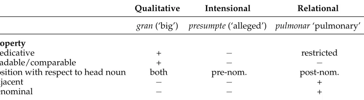
Table 1 summarizes the properties just explained. Our goal is to use these properties to induce the semantic class of adjectives. For instance, if an adjective is denominal, appears almost exclusively in postnominal position, and is strictly adjacent to the head noun, we predict that it is relational. In the experiments reported in Sections 4 and 5, we

Table 1

Initial classification: Linguistic properties of qualitative, intensional, and relational adjectives.

Qualitative Intensional Relational

gran(‘big’) presumpte(‘alleged’) pulmonar‘pulmonary’

Property

predicative + − restricted

gradable/comparable + − −

position with respect to head noun both pre-nom. post-nom.

adjacent − − +

extract data related to these and other properties of adjectives from linguistic resources, and use them as features in machine learning experiments.

3.2 Alternative Classification

In the acquisition experiments reported in Section 5, we distinguish between qualitative, relational, and event-related adjectives. The classification presented in Section 3.1 is thus altered in two ways: (1) The intensional class is dropped. (2) A new class, that of event-related adjectives, is added to the classification. The reasons for these changes will become clear in the discussion of the experiments in Section 4. Here, we describe the newclass and provide a summary table of the alternative classification.

Event-related adjectives. Adjectives such as exportador, prom`es, resultant (‘exporting, promised, resulting’) denote a relationship to an event, in this case,EXPORT,PROMISE, andRESULTevents, respectively. Most of them are deverbal. Like relational adjectives, they are typically nongradable (see Example (8a)) and prefer the postnominal position when modifying nouns (Example (8b)). Like qualitative adjectives, they typically can act as predicates (Example (8c)).

(8) a. ´Es Is

un a

pa´ıs country

{exportador {exporting

/ /

#molt very

exportador} exporting}

de of

petroli oil ‘It is an oil exporting / #very exporting country’ b. #exportador pa´ıs

‘exporting country’ c. Aquest

This pa´ıs country

´es is

exportador exporting ‘This is an exporting country’

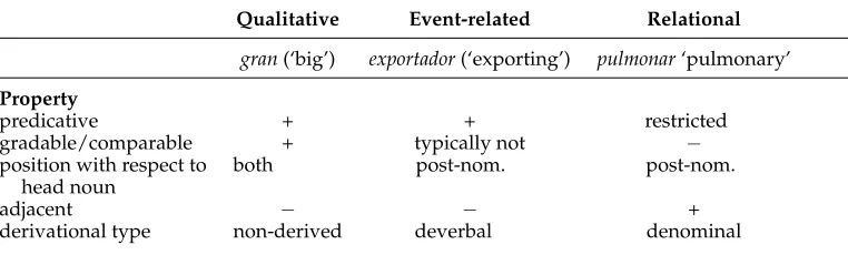
Table 2 summarizes the properties of the alternative classification (for a more thorough discussion of previous research on the semantics of adjectives and more motivation for the classification, see Boleda [2007]). For comparison, we will briefly outline the treatment of adjectives in WordNet (Miller 1998; Alonge et al. 2000). As

Table 2

Alternative classification: Linguistic properties of qualitative, event-related, and relational adjectives.

Qualitative Event-related Relational

gran(‘big’) exportador(‘exporting’) pulmonar‘pulmonary’

Property

predicative + + restricted

gradable/comparable + typically not − position with respect to both post-nom. post-nom.

head noun

adjacent − − +

mentioned in Section 2, the main semantic relation around which adjectives are or-ganized in WordNet is antonymy. Also as explained, however, not all adjectives have antonyms. This is solved in WordNet by the use of indirect antonyms (e.g.,swiftand sloware indirect antonyms, through the semantic similarity betweenswiftandfast). Still, indirect antonymy only applies to a small subset of the adjectives in WordNet (slightly over 20% in WordNet 1.5). Therefore, some kinds of adjectives receive a differentiated treatment.

Specifically, two main kinds of adjectives are distinguished in WordNet: (1) Descrip-tive adjecDescrip-tives, akin to our qualitaDescrip-tive adjecDescrip-tives, which are organized around antonymy (descriptive adjectives, however, include intensional adjectives). (2) Relational adjec-tives, as defined in this article, for which two different solutions are adopted. If a suit-able antonym can be found for a given relational adjective (antonym in a broad sense; in Miller [1998, page 60],physicalandmentalare considered antonyms), it is treated in the same way as a descriptive adjective. Otherwise, it is linked through aPERTAIN-TO pointer to the related noun. In addition, a subclass of descriptive adjectives, having the form of past or present participles, is distinguished, and also receives a hybrid treatment. Those that can be accommodated to antonymy are treated as descriptive adjectives (laughing–unhappy, through the similarity betweenlaughingandhappy). Those which cannot are linked to the source verb through aPRINCIPAL-PART-OFpointer. Our event-related class includes not only past and present participles, but other types of deverbal adjectives. Thus, most of the classes used in this article are to some extent backed up by the organization of adjectives in WordNet.

3.3 The Role of Polysemy

As explained in the Introduction, some adjectives arepolysemoussuch that each sense falls into a different class of the classifications just presented. Consider for instance the adjectiveecon`omic in Example (1), repeated here as Example (9) for convenience. The two main senses of econ`omic instantiate the relational (sense in Example (9a)) and the qualitative class (sense in Example (9b)), respectively.

(9) a. an `alisi econ `omica ‘economic analysis’ b. pantalons econ `omics

‘cheap trousers’

Crucially for our purposes, in each of the senses the adjective exhibits the properties of each of the associated classes. When used as a relational adjective, it is not gradable and cannot be used in a pre-nominal position (Example (10)). When used as a qualitative adjective, it is gradable and it can be used predicatively (see Example (11)). In the experiments that follow, w e aim at capturing this hybrid behavior.

(10) a. #L’an `alisi The-analysis

molt very

econ `omica economic

de of

les the

dades data ‘#The very economic analysis of the data’ b. #Va

‘PAST-AUX dur bring

a to

terme term

una an

econ `omica economic

(11) Aquests These

pantalons trousers

s ´on are

molt very

econ `omics! economic! ‘These trousers are very cheap!’

Cases of regular polysemy between the intensional and qualitative classes also exist, as illustrated in Examples (12) and (13).Antichas two major senses, a qualitative one (equivalent to ‘old, ancient’) and an intensional one (equivalent to ‘former’). Note again that, when used in the intensional sense, it exhibits properties of the intensional class: It appears pre-nominally (Example (13a)) and is not gradable (Example (13b)).

(12) a. edifici building

antic ancient ‘ancient building’ b. edifici

building molt very

antic ancient ‘very ancient building’

(13) a. antic ancient

president president ‘former president’ b. #molt

very antic ancient

president president ‘#very former president’

The newclass in the alternative classification, that of event-related adjectives, also introduces regular polysemy, specifically, between event-related and qualitative adjec-tives, as illustrated in Examples (14) and (15). The participial adjectivesabut(‘known’) has an event-related sense, corresponding to the verbsaber(‘know’), and a qualitative sense that can be translated as ‘wise’. Likewise, the deverbal adjectivecridanerderived fromcridar(‘to shout’) alternates between an event-related sense and a qualitative sense.

(14) problema problem

sabut known

/ /

home man

sabut known ‘known problem / wise man’ (15) noi

boy

cridaner shout_SUFFIX/

/ shirt

camisa

attention-gaining

cridanera

‘boy who shouts a lot / attention-gaining shirt’

Examples (14) and (15) represent cases of regular polysemy because, as can be drawn from the translations, there is a systematic shift from a transparent relation with the event to a quality that bears a more distant relation to the event. In the case ofsabutthe relation is clear (if a man knows a lot, he is wise); in the case ofcridaner, a shirt qualifies for the adjective if it is for instance loud-colored or has an eccentric cut, such that it gains the attention of people, as shouting does.

modified noun than that of the adjective (Pustejovsky 1995). Both of the uses oftrist (‘sad’) illustrated in Example (16) fall into the qualitative class, so, contrary to the work by Lapata (2000, 2001) cited previously, we do not treat the adjective as polysemous in the context of the present experiments.

(16) noi boy

trist sad

/ /

pel·l´ıcula film

trista sad ‘sad boy / sad film’

4. First Model: Polysemous Adjectives Constitute Independent Classes

Given the hybrid behavior of polysemous adjectives explained in Section 3, we can expect that they behave differently from adjectives in the basic classes. For instance, adjectives polysemous between a qualitative and a relational use should exhibit more evidence for gradability than pure relational adjectives, but less than pure qualitative adjectives. In this view, polysemous adjectives belong to a class, for instance, the qualitative-relational class, that is distinct from both the qualitative and the relational classes, typically exhibiting feature values that are in between those of the basic classes. In this section, we report on experiments testing precisely this model for regular polysemy. We will therefore distinguish between five types of adjectives: qualitative, intensional, relational, polysemous between a qualitative and an intensional reading (intensional-qualitative), and polysemous between a qualitative and a relational reading (qualitative-relational). There is one polysemous class missing (intensional-relational). No cases of polysemy between intensional and relational adjectives were observed in our data.

Recall from the previous sections that we cannot reuse an established classification, and that there is virtually no previous work on the automatic semantic classification of adjectives. The present experiments also aim at testing the overall enterprise of inducing semantic classes from distributional properties for adjectives. Given the exploratory nature of the experiment, we use clustering, an unsupervised technique, to uncover natural groupings of adjectives and test to what extent these correspond to the classes described in the literature.

4.1 Data and Gold Standard

The experiments reported in this section are based on an eight million word fragment of the CTILC corpus (Corpus Informatitzat de la Llengua Catalana; Rafel 1994), developed at theInstitut d’Estudis Catalans. Each word is associated with its lemma, part of speech, and inflectional features, as well as syntactic function. Lemma and morphological in-formation have been manually checked. We automatically added syntactic inin-formation with CatCG (Alsina et al. 2002). CatCG is a shallow parser that assigns one or more syntactic functions to each word. In the case of the adjective, CatCG distinguishes between (1) predicate of a copular sentence; (2) predicate in another construction; (3) pre-nominal modifier; (4) post-nominal modifier. As no full dependencies are indicated, the head noun can only be identified with heuristics.

lemmata were chosen token-wise and 50 type-wise to balance high-frequency and low-frequency adjectives (one lemma was chosen with both methods, so the repetition was removed). Two lemmata were added in a post-hoc fashion, as explained subsequently.

The lemmata were annotated by four doctoral students in computational linguistics. The task of the judges was to assign each lemma to one of the five classes (qualitative, intensional, relational, qualitative-intensional, and qualitative-relational). The instruc-tions for the judges included information about all linguistic characteristics discussed in Section 3, including syntactic and semantic characteristics.

The judges had a moderate degree of agreement, comparable to that obtained in other tasks on semantics or discourse, inter-annotator scores ranging betweenκ=0.54 and 0.64 (see Artstein and Poesio [2008] for a discussion of agreement measures for computational linguistics). For comparison, V´eronis (1998) reported a mean pair-wise weightedκ=0.43 for a word sense tagging task in French; and Merlo and Stevenson (2001) obtained κ=0.53–0.66 for the task of classifying English verbs as unergative, unaccusative, or object-drop. Poesio and Artstein (2005) report κ values of 0.63–0.66 (0.45–0.50 if a trivial category is dropped) for the tagging of anaphoric relations. Our judges reported difficulties in tagging particular kinds of adjectives, such as deverbal adjectives. This issue will be retaken in Section 4.5.

No intensional adjectives were identified in the data by the judges, and only one intensional-qualitative adjective was identified. Two intensional lemmata were manually added to be able to minimally track the class. This is clearly insufficient for a quantitative approach, however, so the intensional class is dropped in the alternative classification. It is striking that intensional adjectives, which have traditionally been the focus of formal semantic approaches to the semantics of adjectives, constitute a very small class (less than a dozen lemmata are mentioned in the reviewed literature).

4.2 Features

We use two sets of distributional features to model adjective behavior: on the one hand, theoretically motivated features (theoretical features for short); on the other hand, features that encode the part-of-speech distribution of a four-word window around the adjective (POS features). The former provide a theoretically informed model of adjec-tives, because they are cues to the properties of each class as described in the literature. The latter are meant to provide a theory-independent representation of adjectives, to test to what extent the structures obtained with theoretical and POS features are similar. Both sets of features take a narrowcontext into account (at most five words to each side of the adjective), because of the limited syntactic behavior of adjectives.

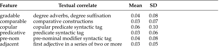
4.2.1 Theoretical Features.Theoretical features model the syntactic and semantic proper-ties of the classes described in Section 3. The features used, together with their mean and standard deviation values (computed on all 3,521 adjectives), are summarized in Table 3. A feature valuev_a,ifor an adjective lemmaaand a featureicorresponds to the proportion of the occurrences in whichiis observed for adjectiveaover all occurrences ofa(see Equation (1);f stands for absolute frequency).

v_a,i= f(a,i)

Table 3 is the translation of Table 1 into shallowcues that can be extracted from a corpus. The mean values in Table 3 are very low, w hich points to the sparseness of theoretically defined properties such as predicativity or gradability, at least in written texts (oral corpora would presumably yield different values). Also note that standard deviations are higher than mean values, which indicates a high variability in the feature values, something that will be exploited for classification.

From the discussion in Section 3, the following predictions with respect to the semantic features can be made.

(1) In comparison with the other classes, qualitative adjectives should have higher values for featuresgradable, comparable, copular, predicative, middle values for featureprenominal, and lowvalues for featureadjacent.

(2) Relational adjectives should have an almost opposite distribution, with very lowvalues for all features except foradjacent.

(3) Intensional adjectives should exhibit very lowvalues for all features except forpre-nominal, for which a very high value is expected.

(4) With respect to polysemous adjectives, it can be foreseen that their feature values will be in between those of the basic classes. For instance, an adjective that is polysemous between a qualitative and a relational reading should exhibit a higher value for featuregradablethan a monosemous relational adjective, but a lower value than a monosemous qualitative adjective.

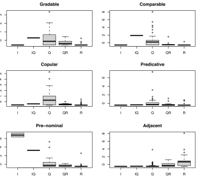
Figure 1 shows that the predictions just outlined are met to a large extent, showing that the empirical (corpus) data support the theoretical predictions. This graph represents the value distribution of each feature in the form of boxplots. In the boxplots, the rectangles have three horizontal lines, representing the first quartile, the median, and the third quartile, respectively. The dotted line at each side of the rectangle stretches to the minimum and maximum values, at most 1.5 times the length of the rectangle. Values that are outside this range are represented as points and termedoutliers(Verzani 2005). Note that the scale in Figure 1 does not range from 0 to 1; this is because the data are standardized, as will be explained subsequently.

Table 3

Theoretical features. The mean and SD values are computed on all clustered adjectives. Feature

copularaccounts for predicative constructions with the copula verbsser, estar(‘be’). Feature

predicativeaccounts for other predicative constructions, such as Example (4d).

Feature Textual correlate Mean SD

Figure 1

Theoretical features: Feature value distribution in the gold standard. Class labels: I = intensional; IQ = polysemous between intensional and qualitative; Q = qualitative; QR = polysemous between qualitative and relational; R = relational.

The differences in value distributions, although significant,1are not sharp, as most of the ranges in the boxes overlap. This affects mainly polysemous classes: Although they showthe tendency predicted—exhibiting values that are in between those of the basic classes—they do not present clearly distinct values. The clustering results will be affected by this distribution, as will be discussed in Section 4.5.

4.2.2 POS Features.POS features encode the part-of-speech distribution of a four-word window around the adjective, providing a theory-independent representation of the linguistic behavior of adjectives. To avoid data sparseness, we encode possible POS for each position as a different feature. For instance, for an occurrence ofalta(‘tall’) as in Ex-ample (17a), the representation would be as in ExEx-ample (17b). In the exEx-ample, the target adjective is in boldface, and the relevant word window is in italics. Negative numbers

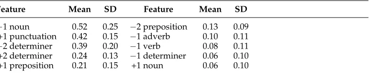
Table 4

POS features. The mean and SD values are computed on all clustered adjectives.

Feature Mean SD Feature Mean SD

−1 noun 0.52 0.25 −2 preposition 0.13 0.09 +1 punctuation 0.42 0.15 −1 adverb 0.10 0.11

−2 determiner 0.39 0.20 −1 verb 0.08 0.11 +2 determiner 0.24 0.13 −1 determiner 0.06 0.10 +1 preposition 0.21 0.15 +1 noun 0.06 0.10

indicate positions to the left, positive ones positions to the right. The representation in Example (17b) corresponds to the parts of speech of´es,m´es,que, andla, respectively.

(17) a. la the

Bruna Bruna

´es is

m´es more

alta tall

que than

l’Angelina the-Angelina ‘Bruna is taller than Angelina’

b. -2 verb, -1 adverb, +1 conjunction, +2 determiner

Feature values are defined as in theoretical features (see Equation (1)). The ten features with the overall highest mean value in our data (among a total of 36 features) are listed in Table 4. Note that the mean values are much higher for the POS features (Table 4) than for the theoretical features (Table 3), as theoretical features are much sparser.

4.3 Clustering Algorithm and Parameters

We use the k-means clustering algorithm (see Kaufman and Rousseeuw[1990] and Everitt, Landau, and Leese [2001] for comprehensive introductions to clustering).2This is a classical algorithm, conceptually simple and computationally efficient, which has been used in related work, such as the induction of German semantic verb classes (Schulte im Walde 2006) and the syntactic classification of Catalan verbs (Mayol, Boleda, and Badia 2005). Also, it performs hard clustering, which is adequate for our purposes (recall from Section 4.1 that we model polysemy in terms of separate classes). Additional experiments with other clustering methods yielded similar results: We tested two hier-archical and one flat algorithm, one of them agglomerative and the other two partitional, with several clustering criteria, always using the cosine distance measure.

K-means is a flat, partitional algorithm that aims at minimizing the overall distance from objects to their centroids (mean vectors of each cluster), which favors globular cluster structures. An initial random partition intokclusters is performed on the data. The centroids (mean vectors) of each cluster are computed, and each object is re-assigned to the cluster with the nearest centroid. The centroids are recomputed, and the process is iterated until no further changes take place, or a pre-specified number of times (20 in our case). Equation (2) shows the formula for the clustering criterion, wherekis the total number of clusters andlare the lemmata in each clusterc1,. . .,ck. To avoid the

influence of the initial partition on the final structure, the whole experiment is repeated several times (25 in our case) with different random partitions, and the partition that better satisfies the clustering criterion is chosen.

minimize

i∈k

l∈ci

cos(l,centroid(ci)) (2)

We experimented with two representations of the feature values: raw and stan-dardized proportions. In clustering, features with higher mean and standard deviation values tend to dominate over more sparse features. Standardization smooths the differ-ences in the strengths of features. We standardize toz-scores, so that all features have mean 0 and standard deviation 1. As the most interpretable results were obtained with standardized values, we will restrict the discussion in the next section to the results obtained with standardized values.

4.4 Results

The discussion focuses on the cluster analyses with three and five clusters because our basis is three classes (intensional, qualitative, and relational) and we consider a total of five classes (basic classes plus polysemous classes: intensional-qualitative and qualitative-relational). A higher number of clusters introduces more noise (in the form of small clusters with no clear content).

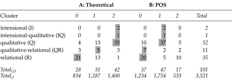
The contingency tables of the clustering results with three clusters are depicted in Table 5. Part A of the table depicts the solution obtained with theoretical features, while Part B represents the solution obtained with POS features. Rows are gold standard classes and columns are clusters, labeled with the cluster number provided by the algorithm. The ordering of the cluster numbers corresponds to the quality of the cluster, measured in terms of the clustering criterion (see Equation (2)), 0 representing the cluster with the highest quality. In each cell Cij of Table 5, the number of adjectives

Table 5

First model: Three-way solution contingency tables for theoretical and POS features. Rows are gold standard classes, columns are clusters. RowTotalGSshows the number of Gold Standard

lemmata and rowTotalclthe total number of lemmata contained in each cluster. Note that the

column labeledTotalrepresents the rowsum for each part (as the number of items per class is identical).

A: Theoretical B: POS

Cluster 0 1 2 0 1 2 Total

intensional (I) 0 0 2 0 2 0 2

intensional-qualitative (IQ) 0 0 1 0 1 0 1

qualitative (Q) 4 13 35 10 37 5 52

qualitative-relational (QR) 3 5 3 7 2 2 11 relational (R) 21 13 1 20 5 10 35

TotalGS 28 31 42 37 47 17 101

of classithat are assigned to clusterjby the algorithm is given. The largest value for each class is highlighted (see gray cells).

A striking feature of Table 5 is that results in the two parts (A and B) are very similar. The following can be observed:

(1) There is one cluster (cluster 0 in both solutions) that contains the majority of relational adjectives in the gold standard. This is the most compact cluster according to the clustering criterion.

(2) Another cluster (2 in solution A, 1 in solution B) contains the majority of qualitative adjectives in the gold standard, as well as all intensional and IQ adjectives.

(3) The remaining cluster contains a mixture of qualitative and relational adjectives in both solutions.

(4) Adjectives that are polysemous between a qualitative and a relational reading (QR) are scattered through all the clusters, although they showa tendency to be ascribed to the relational cluster in solution B (cluster 0).

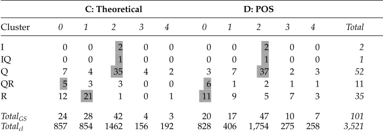
The five-way results are depicted in Table 6. On the one hand, the table shows that the five-way structure found by the clustering algorithm is very similar to the three-way structure in Table 5. This means that the three clusters in A and B have basically been replicated by the three first clusters in C and D, respectively. On the other hand, the differences between the structures obtained using theoretical versus POS features are more obvious in the five-way solutions. From the set-up of the experiment, we had expected one cluster per class, plus QR and IQ adjectives isolated in a cluster of their own. This is clearly not borne out in Table 6. What we find instead is that (a) the mixed clusters persist and score high in the clustering criterion (see clusters 0 in solution C and 0–1 in solution D, with a mixture of Q, QR, and R adjectives), and (b) two additional small clusters are created (clusters 3 and 4 in both solutions) with no clear interpretation, suggesting that the three-way set-up matches better the structure uncovered by the clustering algorithm.

From the discussion of Tables 5 and 6 we conclude that the three-way clustering meets the target classification better than the five-way clustering, and that polysemous adjectives are not identified as a separate class. These results suggest that modeling

Table 6

First model: Five-way solution contingency tables. Information presented as in Table 5.

C: Theoretical D: POS

Cluster 0 1 2 3 4 0 1 2 3 4 Total

I 0 0 2 0 0 0 0 2 0 0 2

IQ 0 0 1 0 0 0 0 1 0 0 1

Q 7 4 35 4 2 3 7 37 2 3 52

QR 5 3 3 0 0 6 1 2 1 1 11

R 12 21 1 0 1 11 9 5 7 3 35

TotalGS 24 28 42 4 3 20 17 47 10 7 101

polysemous adjectives in terms of additional, complex classes is not an adequate strat-egy (we return to this point subsequently).

Recall that we defined theoretical and POS features to compare the structures obtained using theoretically informed and theory-independent features. Further feature analysis, not reported here for space reasons, reveals a high correlation between the most descriptive features of solutions A and B.3 This highlights the correspondence between the two feature representations with respect to the clustering results: The POS features elicited as most discriminative by the clustering algorithm are precisely those that correspond to the theoretical features. This correspondence explains the resemblance between the solutions obtained with the two types of representation and at the same time provides support for the present definition of the theoretical features.

Last but not least, note that we do not assign a score to each clustering solution. Evaluation of clustering is very problematic when there is no one-to-one correspon-dence between classes and clusters (Hatzivassiloglou and McKeown 1993), as is our case. Schulte im Walde (2006) provides a thorough discussion of this issue and proposes different metrics and types of evaluation. We defer numerical evaluation until Section 5.

4.5 Discussion

4.5.1 Classification.The experiments presented provide feedback to the question, what is an appropriate broad semantic classification for adjectives? The clustering experiments provide empirical support for the qualitative and relational classes, as is particularly evident in the three-way solution (Table 5). These are classes that have traditionally been taken into account in descriptive grammar (Bally 1944; Picallo 2002) and computational resources such as WordNet (Miller 1998; Alonge et al. 2000), so we consider them to be quite stable and keep them in our classification.

Intensional and IQ adjectives, in contrast, are grouped together with qualitative adjectives in all solutions, because they do not exhibit distinctive enough distributional properties to differentiate them, a fact aggravated by the small size of the intensional class. From the point of viewof NLP, it is reasonable to encode intensional adjectives by hand, given their limited number. For these reasons, we include the intensional class in the qualitative class in what follows (remember that, as mentioned in Sec-tion 3, WordNet also includes intensional adjectives in the qualitative—in their terms, descriptive—class).

”Hybrid” clusters, that is, clusters that contain adjectives from several semantic classes, play an interesting role in our cluster analyses. Such clusters seem to be coherent and stable, as they appear in all examined solutions (A, B, and also C and D in Tables 5 and 6) and have good scores in the clustering criterion. Significantly, however, most of the adjectives that are problematic for humans are assigned to hybrid clusters, where problematic means that they are not assigned to the same class by all four judges. Conversely, most adjectives in the hybrid clusters are problematic. Thus, hybrid clusters are useful to signal problems in the proposed classification. As an example, consider cluster 0 in Part C of Table 6: 17 out of the 24 (70.1%) gold standard adjectives in this hybrid cluster are problematic for humans. This cluster contrasts with the qualitative cluster (cluster 2 of Table 6), where only 10 out of its 42 (23.8%) lemmata are problematic. Two kinds of adjectives crop up among problematic adjectives: so-called ethnic adjectives (alemany ‘German’, menorqu´ı ‘Menorcan’, sud-afric`a ‘South African’, xin`es

‘Chinese’), and deverbal adjectives (indicador‘indicating’, parlant‘speaking’, protector ‘protecting, protective’, salvador ‘savior’). Ethnic adjectives can act as predicates of copular sentences in a much more natural way than typical relational adjectives, and seem to be vague between a relational and a qualitative reading in their semantics (Raskin and Nirenburg 1998, page 173). This kind of adjective will mainly be treated as polysemous in the experiments reported in Section 5.

As for deverbal adjectives, they are clearly neither relational (they do not express a relationship to an object) nor intensional. They are also not typically qualitative, however, because they trigger a relationship to an event instead of denoting a simple property. For instance,protectortriggers a relationship with a stable event of protecting in Example (18): A person namedSerrabelongs to the kind of associates who have as a primary role toprotectthe association.

(18) Serra Serra

. . . Era . . . w as

soci associate

protector protecting

de of

l’Associaci ´o the-Association

de of

concerts concerts ‘Serra was a protecting associate of the Association of concerts’

These considerations motivate the addition of a class of event-related adjectives in the overall classification. Event-related adjectives have not received much attention in the linguistic literature, except for one particular subtype, namely, adjectival uses of the participle (Bresnan 1982; Levin and Rappaport 1986; Bresnan 1995). As for compu-tational resources, the English WordNet, as explained in Section 3, only distinguishes some participial adjectives. In the Italian WordNet, however, other event-related adjec-tives receive a specific treatment, through the encoding of the lexical relationsCAUSES andLIABLE-TO, as exemplified in Example (19) (Alonge et al. 2000):

(19) a. depuratorio‘depurative, purifying’CAUSESdepurare‘to depurate/purify’. b. giudicabile‘triable’LIABLE-TOgiudicare ‘to judge’.

To sum up, the results of the experiments reported in this section motivate a three-way classification between qualitative, event-related, and relational adjectives. Note that, in the revised classification proposed in this section, classes are uniformly defined according to the ontological typeof their denotation: Qualitative adjectives denote at-tributes or properties, relational adjectives denote relationships to objects, and event-related adjectives denote relationships to events. The classes correspond to the three major types of entities in an ontology (attributes, objects, events), more specifically, to the way adjectives participate from those entities. In this view, relational and event-related adjectives denote properties, just as qualitative adjectives do, but they are a specific type of property involving a relationship with either an object or an event. The classification is in fact similar to the one proposed in the Ontological Semantics framework (Raskin and Nirenburg 1998; Nirenburg and Raskin 2004).

such asaudible orablaze. Similarly, some object adjectives are not denominal (such as bot`anic‘botanical’). Conversely, some denominal or deverbal adjectives are qualitative: vergony´os ‘shy’ (from vergonya ‘shyness’), amable (literally ‘suitable to be loved’; has evolved to ‘kind, friendly’). We will empirically check the correspondence between morphology and semantic class in Section 5.5.

4.5.2 Regular Polysemy. Our first series of experiments also provides feedback to the question, what is an adequate computational model for regular polysemy? Specifically, we have shown that the treatment of regular polysemy in terms of independent classes is not adequate. Remember that the motivation for the experiments presented in this section was the hypothesis that polysemous adjectives exhibit a linguistic behavior that participates from the basic classes involved in the regular polysemy, thus yielding feature values that are in between those of the basic classes (cf. Figure 1). Thus, we had expected that polysemous adjectives form a homogeneous group of lexical items, char-acterized precisely by the fact that they exhibit properties from each class to a certain degree. However, this expectation is not borne out in the results of the experiments. To this respect, it is striking that QR adjectives (polysemous between a qualitative and a relational reading) are spread throughout all the clusters in all solutions. They are not identified as a homogeneous group, nor as distinct from the rest. Crucially, as pointed out in Section 4.2, the differences between the feature values of polysemous adjectives and those of the basic classes are not strong enough to motivate a separate cluster.

We believe that the reason for these results is the fact that polysemous adjectives do notin fact have a homogeneous, differentiated profile: In a given corpus, most adjec-tives are used predominantly in one of their senses, corresponding to one of the basic classes, and thus the “hard” classification with three clusters fits better. For instance, the qualitative-relational adjectiveir`onic(‘ironic’) is mainly used as a qualitative adjective in the corpus. Accordingly, it always appears in the qualitative clusters. Conversely, militar(‘military’) is mostly used as a relational adjective, and is consistently assigned to one of the relational clusters in all solutions. Thus, although polysemous adjectives on average do showa mixed behavior, each lexical item tends to pattern with one of the basic classes. An alternative conceptualization of regular polysemy and experimental design is called for, and this will be the topic of the next section.

5. Second Model: Polysemous Adjectives Simultaneously Belong to Different Classes

The experiments presented in the previous section pursued two goals: on the one hand, to test the initial classification proposal; on the other, to test a model of regular polysemy that treats polysemous adjectives in terms of separate classes. With respect to the first goal, the experiments in this section rely on the results of the previous experiments, and use the alternative classification described in Section 3.2. The alternative classification has in addition been supported by a clustering experiment not reported here for space reasons (see Boleda, Badia, and Batlle [2004] for details and discussion).

adjectives: the fact that they are used predominantly in one of their senses, and the fact that the feature distributions of “polysemous classes” largely overlap with those of the basic classes.

In the present experiments, we develop an alternative approach to regular poly-semy that is based on the perspective that polysemous adjectives belong to more than one semantic class, in the framework ofmulti-label classification. A typical example of a multi-label classification task is Text Categorization (Schapire and Singer 2000), where a document can be described via more than one label (e.g.,HealthandLocal), so that it effectively belongs to more than one of the target classes. The motivation for this newapproach is the fact that polysemous adjectives exhibit properties of all the classes involved (see Section 3.3). The hypothesis is that the evidence found for a polysemous adjective that is polysemous between, say, a relational and a qualitative use should be strong enough for the adjective to be assigned to both the relational and the qualitative classes. Note that by assigning the adjective to the two classes independently, we make animplicitclassification of the adjective as polysemous. The success of the approach will depend on whether the different senses are sufficiently represented in the data, and it will be especially challenging to distinguish between noise and evidence for a given class.

5.1 Data and Gold Standard

The experiments reported in this section are based on a 16 million word fragment of the CTILC corpus (see Section 4.1). We additionally use an adjective database (Sanrom `a and Boleda 2010) with manually coded information about all adjectives occurring more than 50 times in the corpus (2,296 lemmata). The database codes the derivational type (deverbal, denominal, participial, non-derived) and suffix of each adjective.

A gold standard of 210 adjective lemmata (available in the Appendix) was selected from this database for the experiments. The lemmata were randomly sampled in a stratified fashion, balancing three factors of variability: frequency, morphological type, and suffix. Thus, the gold standard contains an equal number of adjectives from three frequency bands (low, medium, high), from the four derivational types, and from a series of suffixes within each type. This sampling method is aimed at achieving semantic variability.

Three experts assigned each of the 210 lemmata to one or two of the classes in the alternative classification, namely, event-related, qualitative, or relational. The decisions were reached by consensus and were based on expert knowledge together with the examination of the information in the database, corpus examples, and the judgments provided by 322 naive subjects in a large-scale annotation experiment.4

Table 7 shows the distribution of adjectives in the gold standard into classes ac-cording to the three experts. These are the data used in the experiments presented in this section. The proportion of polysemous adjectives is quite high, over 17%, with qualitative-relational being the most frequent type of polysemy. Also note that 51% of the adjectives are qualitative; this will be the baseline for the machine learning experiments presented subsequently.

Table 7

Gold standard classification: Distribution and examples.

Class Label Example # %

qualitative Q tena¸c, ‘tenacious’ 107 51.0 event E informatiu, ‘informative’ 37 17.6 relational R crani`a, ‘cranial’ 30 14.3 qualitative-relational QR familiar, ‘familiar’ 23 11.0 qualitative-event QE sabut, ‘known’ 7 3.3 event-relational ER comptable, ‘countable’ 6 2.9

Total 210 100

Table 8

Feature sets. From left to right, each column depicts, for each feature set, an identifier, a description of the type of information used, the total number of features, and one example feature. Feature setmorphcontains two categorical features that are transformed into 25 if binarization is applied; the remaining feature sets are numerical.

Feature set Description # Example

morph morphological (derivational) properties 2 (25) suffix

func syntactic function of the adjective 4 post-nom. modifier

uni uni-gram POS (1 word to left or to right) 24 −1noun

bi bi-gram POS (1 word to left and 1 to right) 50 −1noun+1adj

theor distributional cues of theoretical properties 18 gradable

Total 98 (121)

5.2 Features

5.2.1 Feature Definition.We define five feature sets based on different types of linguistic information, to gain further insight into the properties of each class. In particular, we are interested in the properties of event-related adjectives, for which we do not have a description in the linguistic literature. Table 8 summarizes the properties of the feature sets used for the present experiments.

Feature set morph represents derivational properties of adjectives, as encoded in the adjective database. We include this type of information because of the relevance of morphology for the newclassification (see Section 4.5). Funcencodes the syntactic functions of the adjectives in the corpus, as explained in Section 4.1.Uni(forunigram) and bi (for bigram) encode the distribution of the adjective in the corpus in terms of the parts of speech of the surrounding words. Feature analysis of the first experiment showed that the word preceding and following the target were the most informative, so in the present experiment only a one-word window is taken into account. The unigram distribution (uni) encodes each part of speech separately, as was done in the first experiment, and the bigram distribution (bi) takes the left and right word jointly, to avoid feature correlation effects. In the latter feature set, only the 50 most frequent bigrams are considered, to avoid features that are too sparse.5

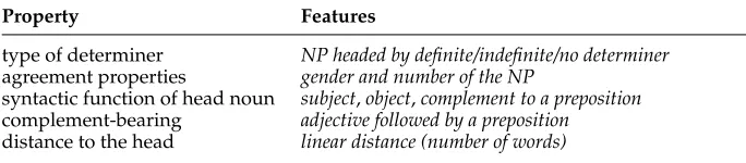
Table 9

Newor revised features in feature settheor. Each rowlists the property we aim to capture and the features through which the property is encoded. The information relies on the information in the corpus, which does not include full syntactic structure.

Property Features

type of determiner NP headed by definite/indefinite/no determiner

agreement properties gender and number of the NP

syntactic function of head noun subject,object,complement to a preposition

complement-bearing adjective followed by a preposition

distance to the head linear distance (number of words)

Finally, feature set theor (for theoretical) generalizes and adds to the theoretical properties used in the first experiment (Table 3 in Section 4.2). Upon inspection of the clustering solutions (not reported here for space reasons), some further potentially relevant distributional pieces of information cropped up that were included in the theor features of the present experiment. The newfeatures, summarized in Table 9, cover several aspects of the noun phrases (NPs) in which adjectives occur: The type of determiner of the NP, agreement properties (as these can correlate with semantic properties), the syntactic function of the head noun, and the presence of a potential adjective complement. The latter are usually headed by prepositions (El Joan est`a gel´os d’en Pere, ‘Joan is jealous of Pere’). Finally, featuredistance to the headis a reformulation of feature adjacent from Section 4.2. It encodes the mean distance of the adjective to the head, in number of words, as this is a more general definition that alleviates data sparseness.

As for feature values, they are computed as in the first experiment (see Equation (1)), with the following exceptions: (1)morphfeatures are of categorical type, so their values are not numerical; (2) the two first features in Table 9, due to data sparseness consider-ations, are computed as proportions over the use of the adjective as a nominal modifier (see Equation (3), wherea_modis the number of occurrences of the adjective as modifier); (3) the values for featuredistance to the head, also in Table 9, do not range from 0 to 1 as the other feature values, because they correspond to the mean distance to the head in number of words. The data set used for the present experiments is available at the ACL repository.6

va,i=

f(amod,i)

f(a_mod) (3)

5.2.2 Feature Tuning.We test the effects of feature selection in the performance of the classifiers. The features are selected according to their performance within the machine learning algorithm used for classification. Accuracy for a given subset of features is estimated by cross-validation over the training data. Because the number of subsets in-creases exponentially with the number of features, this method is computationally very expensive, so we use a best-first search strategy. We also experiment with binarization of the two categorical features (suffix,derivational type).

5.3 Method

The classification task is approached with a two-level architecture.

1. The decision on the class of the adjective is decomposed into threebinary decisions: Is it qualitative or not? Is it event-related or not? Is it relational or not?

2. A complete classification is achieved bymergingthe results of the binary decisions. A consistency check is applied by which (a) if all decisions are negative, the adjective is assigned to the qualitative class (the most frequent one; this was the case for a mean of 4.6% of the class assignments); (b) if all decisions are positive, we randomly discard one (three-way polysemy is not foreseen in our classification; this was the case for a mean of 0.6% of the class assignments).

This is the standard architecture for multi-label classification tasks (Schapire and Singer 2000; Ghamrawi and McCallum 2005), and it has also been applied to NLP problems such as entity extraction and noun-phrase chunking (McDonald, Crammer, and Pereira 2005).

Note that in the present experiments we change both the classification and the approach (unsupervised vs. supervised) with respect to the first set of experiments presented in Section 4, which can be seen as a sub-optimal technical choice. After the first series of experiments that required a more exploratory analysis, however, we believe that we have now reached a more stable classification, which we can test by supervised methods. In addition, we need a one-to-one correspondence between gold standard classes and clusters for the approach to work, which we cannot guarantee when using an unsupervised approach that outputs a certain number of clusters with no mapping to the gold standard classes.

We test two types of classifiers. The first type are Decision Tree classifiers trained on different types of linguistic information coded as feature sets. Decision Trees are one of the most widely machine learning techniques (Quinlan 1993), and they have been used in related work (Merlo and Stevenson 2001). They have relatively few parameters to tune (a requirement with small data sets such as ours) and provide a transparent representation of the decisions made by the algorithm, which facilitates the inspection of results and the error analysis. We will refer to these Decision Tree classifiers assimple classifiers, in opposition to the ensemble classifiers, which are complex, as explained next.

of “strange” class assignments made by one single classifier, which are therefore overridden by the class assignments of the remaining classifiers.7

For the evaluation, 100 different estimates of accuracy are obtained for each feature set using 10-run, 10-fold cross-validation (10x10 cvfor short). In this schema, 10-fold cross-validation is performed 10 times, that is, 10 different random partitions of the data (runs) are made, and 10-fold cross-validation is carried out for each partition. To avoid the inflated Type I error probability when reusing data (Dietterich 1998), the significance of the differences between accuracies is tested with thecorrected resampled t-testas proposed by Nadeau and Bengio (2003).8

5.4 Results

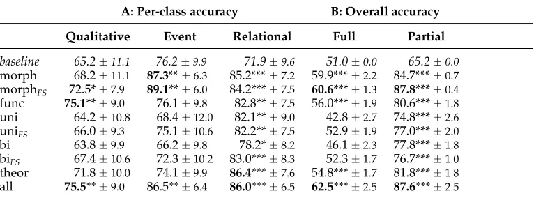
5.4.1 Simple Classifiers.The accuracies for the simple classifiers are shown in Table 10. Part A of the table lists the results for each of the binary decisions (qualitative/ non-qualitative, event/non-event, relational/non-relational). The accuracy for each de-cision is computed independently. For instance, a qualitative-event adjective is judged correct within the qualitative class iff the decision isqualitative; correct within the event class iff the decision isevent; and correct within the relational class iff the decision is non-relational.

Part B reports the accuracies for the overall, merged class assignments, taking polysemy into account (qualitative vs. qualitative-event vs. qualitative-relational vs. event, etc.).9In Part B, we report two accuracy measures: full and partial. Full accuracy requires the class assignments to be identical (an assignment of qualitative for an adjec-tive labeled as qualitaadjec-tive-relational in the gold standard will count as an error), whereas partial accuracy only requires some overlap in the classification of the machine learning algorithm and the gold standard for a given class assignment (a qualitative assignment for a qualitative-relational adjective will be counted as correct). The motivation for reporting partial accuracy is that a class assignment with some overlap with the gold standard is more useful than a class assignment with no overlap. The figures in the discussion that followrefer to full accuracy unless otherwise stated.

For the qualitative and relational classes, taking into account distributional infor-mation allows for an improvement over the default morphology–semantics mapping outlined in Section 4.5: Feature setall, containing all the features, achieves 75.5% accu-racy for qualitative adjectives; feature settheor, with carefully defined features, achieves 86.4% for relational adjectives. In contrast, morphology seems to act as a ceiling for

7 The experiments discussed in this section were carried out with the Weka software package (Witten and Frank 2011), version 3.6. The Decision Tree algorithm used is J48, the latest open source version of C4.5 (Quinlan 1993), with default parameters (binary splits= False,confidence factor for pruning= 0.25,

minimum number of instances per leaf= 2,reduced-error pruning= False,subtree raising= True,unpruned= False,use Laplace= False). AdaBoost has also been used with default parameters (base classifier= Decision Stump,number of iterations= 10,random seed= 1,use resampling instead of reweighting= False,weight threshold= 100). For Attribute Bagging, we used the Random Subspace algorithm, with J48 as base classifier (parameters as before),bag size= 1/3, andrandom seed= 1. We experimented with different values for the number of iterations (see Section 5.4.2).

8 Note that the corrected resampled t-test can only compare accuracies obtained under two conditions (algorithms or, as is our case, feature sets); ANOVA would be more adequate. In the field of machine learning, there is no established correction for ANOVA for the purposes of testing differences in accuracy (Bouckaert 2004). Therefore, we use multiple t-tests instead, which increases the overall error probability of the results for the significance tests.