900
Global Autoregressive Models for Data-Efficient Sequence Learning
Tetiana Parshakova Stanford University⇤ [email protected]
Jean-Marc Andreoli Naver Labs Europe
{jean-marc.andreoli,marc.dymetman}@naverlabs.com Marc Dymetman Naver Labs Europe
Abstract
Standard autoregressive seq2seq models are easily trained by max-likelihood, but tend to show poor results under small-data condi-tions. We introduce a class of seq2seq mod-els, GAMs (Global Autoregressive Models), which combine an autoregressive component with a log-linear component, allowing the use of globala priorifeatures to compensate for lack of data. We train these models in two steps. In the first step, we obtain an unnormal-izedGAM that maximizes the likelihood of the data, but is improper for fast inference or eval-uation. In the second step, we use this GAM to train (by distillation) a second autoregres-sive model that approximates thenormalized distribution associated with the GAM, and can be used for fast inference and evaluation. Our experiments focus on language modelling un-der synthetic conditions and show a strong per-plexity reduction of using the second autore-gressive model over the standard one.
1 Introduction
Neural sequential text generation models have become the standard in NLP applications such as language modelling, NLG, machine transla-tion. When enough data is available, these mod-els can be trained end-to-end with impressive re-sults. Generally, inference and training proceed in an auto-regressive manner, namely, the next decoded symbol is predicted by a locally nor-malized conditional distribution (the “softmax”). This has several advantages: (i) the probability of the sequence is already normalized, by the chain-rule over local decisions, (ii) max-likelihood (ML) training is easy, because the log-likelihood of the full sequence is simply the sum of local CE (cross-entropy) losses, (iii) exact sampling of full
se-⇤Work conducted during an internship at NAVER Labs
Europe.
quences from the model distribution is directly ob-tained through a sequence of local sampling deci-sions.
However, these autoregressive models (AMs) tend to suffer from a form of myopia. They have difficulty accounting for global properties of the predicted sequences, from overlooking certain as-pects of the semantic input in NLG to duplicating linguistic material or producing “hallucinations” in MT, and generally through being unable to ac-count for long-distance consistency requirements that would be obvious for a human reader.1
The main contributions of this paper are as fol-lows.
First, we propose a hybrid seq2seq formaliza-tion, the Global Autoregressive Model (GAM), that combines a local autoregressive component with a global log-linear component, allowing the use ofa priorifeatures to compensate for the lack of training data. GAMs are related both to the class of Energy-Based Models (EBM) and to that of Exponential Families (EF), and inherit some important properties from those: an intimate re-lationship between training and sampling (EBM); the identity of empirical and model expectations at maximum-likelihood; convexity of log-likelihood (EF).
and evaluation.
Third, we demonstrate the ability of GAMs to be data-efficient, namely, to exploit the original data better than a standard autoregressive model. In order to clarify the core techniques and issues, we design a simple class of synthetic data, con-sisting of random binary strings containing “mo-tifs” (specific substrings) that we can manipulate in different ways. We show that, in limited data conditions, GAMs are able to exploit the features to obtain final autoregressive models that perform better than the original ones.
The remainder of the paper is structured as fol-lows. In Section 2, we provide some background about autoregressive models, energy-based mod-els, and log-linear models. In Section 3, we intro-duce GAMs. In section 4, we describe our focus on synthetic data. In Section 5, we explain our training procedure. In Section 6, we comment on related work. In Section 7, we describe our ex-periments. In Section 8, we provide an analysis of our results. We conclude with a discussion in Section 9. Note that some additional explanations and experiments are provided in the Supplemen-tary Material, indicated by [SM].
2 Background
2.1 Autoregressive models (AM)
These are currently the standard for neural seq2seq processing, with such representatives as RNN/LSTMs (Hochreiter and Schmidhuber,
1997;Sutskever et al.,2014), ConvS2S (Gehring et al.,2017), Transformer (Vaswani et al.,2017)). Formally, they are defined though a distribution r⌘(x|C), where C is an input (aka Context, e.g.
a source sentence in Machine Translation (MT)), andxis a target sequence (e.g. a target sentence in MT). We have:
r⌘(x|C)=.
Y
i
s⌘(xi|x1, . . . , xi 1, C),
where each s⌘(xi|x1, . . . , xi 1, C) is a
normal-ized conditional probability over the next symbol of the sequence, computed by a neural network (NN) with parameters⌘. The local normalization of the incremental probabilities implies the over-all normalization of the distributionr⌘(x|C), and
consequently, the possibility of directly sampling from it and evaluating the likelihood of training sequences.
2.2 Energy-Based Models (EBM)
EBMs are a generic class of models, characterized by an energy functionU⌘(x|C)computed by a NN
parametrized by ⌘ (LeCun et al., 2006). Equiva-lently, they can be seen as directly defining a po-tential (an unnormalized probability distribution) P⌘(x|C) = e U⌘(x|C), and indirectly the
normal-ized distribution p⌘(x|C) = 1/Z⌘(C) P⌘(x|C),
with Z⌘(C) = PxP⌘(x|C). A
fundamen-tal property of these models is that, for max-likelihood training, the SGD updates can be com-puted through the formula:2
r⌘logp⌘(x|C) =r⌘logP⌘(x|C) (1)
Ex⇠p⌘(·|C)r⌘logP⌘(x|C),
which, in principle, reduces the problem of train-ing with unnormalized potentials to the problem ofsamplingfrom them.
2.3 Log-Linear Models / Exponential Families
Log-Linear models (Jebara, 2013) are the con-ditional version of Exponential Families (Jordan,
2010). The general form of a log-linear model (for the discrete case) is as follows:
p (x|C) = 1/Z (C)µ(x;C)eh (C), (x;C)i,
withZ (C) = Pxµ(x;C)eh (C), (x;C)i. Here (x;C)is a vector of predefined real features of the pair(x, C), which is combined by scalar prod-uct with a real vector of weights (C)of the same dimension; µ(x;C) is an arbitrary “base mea-sure”, which is fixed. These models, which al-low to introduce prior knowledge through features and have nice formal properties (see below), were mainstream in NLP before the revival of neural ap-proaches.
3 Proposal: GAMs
We now define Global Autoregressive Models
(GAMs). These are hybrid seq2seq models that exploit both local autoregressive properties as well as global properties of the full target sequence. A GAM is an unnormalized distributionP⌘(x|C)
over sequencesx, parametrized by a vector⌘ = ⌘1 ⌘2:
P⌘(x|C) =r⌘1(x|C)·eh ⌘2
(C), (x;C)i. (2)
Herer⌘1(x|C)is an autoregressive seq2seq model
for generating x from input C, parametrized by ⌘2; (x;C)is a vector of predefined real features
of the pair(x, C), which is combined by a scalar product with a real vector ⌘2(C)of the same
di-mension, computed over the inputCby a network parametrized by ⌘2. The normalized distribution
associated with the GAM isp⌘(x|C) = PZ⌘⌘(x(C|C)),
whereZ⌘(C) =PxP⌘(x|C).
GAMs appear promising for the following rea-sons:
• Features (x;C)provide a simple way to draw attention of the model to potentially useful as-pects that may be difficult for the AM compo-nent to discover on its own from limited data.
• GAMs are an instance of EBMs, where the po-tential P⌘(x|C) is the product of the an AM
potentialr⌘1(x|C)with a “log-linear” potential
eh ⌘2(C), (x;C)i. Here the gradient relative to the log-linear part takes the especially simple form:
r⌘2logp⌘(x|C) = (x;C) (3)
Ex⇠p⌘(·|C) (x;C).
• Log-linear models, on their own, while great at expressing prior knowledge, are not as good as AM models at discovering unforeseen regular-ities in the data. Also, they are typically prob-lematic to train from a log-likelihood perspec-tive, because sampling from them is often un-feasible. GAMs address the first issue through thercomponent, and alleviate the second issue by permitting the use ofr as a powerful “pro-posal” (aka “surrogate”) distribution in impor-tance sampling and related approaches, as we will see.
4 Experimental focus
While the motivation for GAMs ultimately lies in practical NLP applications such as those evoked earlier, in this paper we aim to understand some of their capabilities and training techniques in simple and controllable conditions. We focus on the un-conditional (i.e. language modelling) case, and on synthetic data. Our setup is as follows:
• We consider an underlying process ptrue that generatesbinary sequencesaccording to a well-defined and flexible process. In this paper we use PFSAs (Probabilistic Finite State Au-tomata) to impose the presence or absence of
sub-strings (“motifs”) anywhere in the gener-ated data, exploiting the intersection properties of automata.
• Due to the dynamic programming properties of PFSAs, it is possible to compute the true en-tropy H(ptrue) = Pxptrue(x) logptrue(x) of the process (see [SM]), as well as other quantities (Partition Functions, Mean sequence length); it is also possible to generate training (D), validation (V), and test data (T) in arbi-trary quantities.
• We employ an unconditional GAM of the sim-ple form:
p (x)=. P (x)
Z ,withZ
.
=X
x
P (x)and
P (x)=. r(x)·eh , (x)i, (4)
whereris trained onDand then kept fixed, and where is then trained on top ofr, also onD.
It should be noted that with r fixed in this way, this formulation exactly corresponds to the definition of an exponential family (Jordan,
2010), with r asbase measure. In such mod-els, we have two important properties: (i) the log-likelihood of the data is convex relative to the parameters , and thus a local maximum is also global; (ii) the max-likelihood value
⇤ has the property that the model expectation
Ex⇠p ⇤(·) (x)is equal to the empirical expec-tation|D| 1P
x2D (x)(“Moment Matching” property of exponential families).
• We are specially interested in the relative data-efficiencyof the GAM compared to the AM r: namely the ability of the GAM to recover a lower perplexity approximation ofptruethanr, especially in small training-set conditions.
5 Training procedure
5.1 Two-stage training
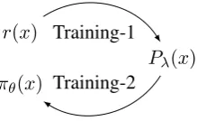
r(x)
⇡✓(x)
P (x)
Training-1
[image:4.595.127.237.68.135.2]Training-2
Figure 1: Two-stage training. At the end of the pro-cess, we compare the perplexities ofrand⇡✓ on test
data:CE(T, r)vs.CE(T,⇡✓).
Training-1 This consists in training the model P onD. This is done by first trainingr onDin the standard way (by cross-entropy) and then by training by SGD with the formula (adapted from (3)):
r logp (x) = (x) Ex⇠p (·) (x). (5)
The main difficulty then consists in computing an estimate of the model momentsEx⇠p (·) (x). In
our experiments, we compare two Monte-Carlo approaches (Robert and Casella, 2005) for ad-dressing this problem: (i)Rejection Sampling(rs), using r as the proposal distribution and (ii)
Self-Normalized Importance Sampling (snis) (Owen,
2017;Y. Bengio and J. S. Senecal,2008), also us-ingras the proposal.
Rejection sampling is performed as follows. We use r(x) as the proposal, and P (x) = r(x) e · (x) as the unnormalized target distribu-tion; for any specific , because our features are bounded between 0 and1, we can easily upper-bound the ratio P (x)
r(x) = e · (x) by a number
; we then sample x from r, compute the ratio ⇢(x) = Pr((xx)) 1, and acceptxwith probability ⇢(x). The accepted samples are unbiased samples fromp (x)and can be used to estimate model mo-ments.
Snis also uses the proposal distribution r, but does not require an upper-bound, and is directly oriented towards the computation of expectations. In this case, we sample a number of points x1, . . . , xN fromr, compute “importance ratios” w(xi) = Pr((xxii)), and estimate Ex⇠p (·) (x)
throughEˆ= PiPw(xi) (xi)
iw(xi) . The estimate is biased
for a givenN, but consistent (that is, it converges to the trueE forN ! 1).
Training-2 While Training-1 results in a well-defined model P (x), which may fit the data closely in principle, we should not conclude
that P (x) is convenient to use for inference — namely, in language modeling, efficiently sam-pling from its normalized version p (x); as seri-ously, because of the partition factorZ , it is also not obvious toevaluatethe perplexity ofP (x)on test data. In order to do both, one approach con-sists in using adistillationtechnique (Hinton et al.,
2015), where, during training, one expends gener-ous time towards producing a set of samples from P , for instance by Monte-Carlo (e.g. Rejection Sampling) techniques, and where this set (which may be arbitrarily larger than the original D) is in turn used to train a new autoregressive model ⇡✓(x), which can then be used directly for
sam-pling or for computing data likelihood. This is the approach that we use in our current experiments, again using the originalr(x)as a proposal distri-bution.
5.2 Cyclical training
In the case of small|D|, the proposal distribution r is weak and as a result the distillation process, based on rejection sampling, can be slow. To ad-dress this issue, we also consider a cyclical train-ing regime that updates the proposal distribution after distilling each batch of samples, with the in-tention of reducing the rejection rate. Once the process of distillation is finished, we use the aggre-gated samples to train the final⇡✓. The two-stage
training procedure is a variant of the cyclical one, with a fixed proposal (see Algorithm 1 for more details).
6 Related Work
(Hoang et al., 2018), working in a NMT con-text, have a similar motivation to ours. They first train an autoregressive seq2seq model (Trans-former in their case) on bilingual data, then at-tempt to control global properties of the generated sequences through the introduction of a priori fea-tures. They interpolate the training of the autore-gressive model with training of a Moment Match-ing component which tries to equate the features expectations of the model with those of the data. Contrarily to our approach, they do not directly try to maximize likelihood in an integrated model.
Algorithm 1Training
1: functionTRAIN(D, V, T, f t, DsSize, tReg, mode)
2: r TRAINRNN(D, V,optAdam) .initialize and then train RNN
3: P TRAINGAM(r, D, V,tReg, f t) .train for a given proposalr
4: ifmode=‘two stage’then .Training-2: distill in one step 5: D,e V ,e DISTILLBATCH(P ,DsSize)
6: else ifmode=‘cyclic’then .Cyclic-training: distill in several steps 7: De {};Ve {};flag False
8: while|De|<DsSizedo .proceed to the distillation process
9: DB,e VB,e accptRate DISTILLBATCH(P ,bSize) .accptRate - acceptance rate ofrsduring distillation 10: De.insert(DBe );Ve.insert(VBe )
11: if notflag then
12: r SINGLEUPDATERNN(r,DB,e optAdam) .improve proposalr
13: P TRAINGAM(r, D, V,tReg, f t) .train for a given proposalr
14: flag EARLYSTOPPINGd(acceptRate) .check if acceptance rate has stopped improving 15: De.insert(D);Ve.insert(V) .add true data to the distilled one 16: ⇡✓ TRAINRNN(D,e V ,e optAdam)
17: return⇡✓
18:functionTRAINGAM(P , D, V, tReg,f t) .Training-1
19: ↵0 10 .initial learning rate
20: target mom GETMOMENTS(D, V, ft) .empirical moments of the given dataset 21: while notEARLYSTOPPING(`1mom)do .check if`1momhas stopped improving
22: model mom [0]⇥|f t| .accumulate the model’s moments
23: ↵t 1+#epoch↵0
24: forb2range(#updatesPerEpoch)do
25: mean mom GETMOMENTSGAM(P , D, V,tReg, f t) .usersorsnisto estimateEx⇠p (·) (x)
26: model mom (model mom+mean mom/(b 1))·b 1
b .moving average
27: r target mom mean mom .use Eq.5to compute gradients
28: +↵t·r
29: `1mom ktarget mom model momk1
30: returnP
focus on inference as maximization, e.g. finding the best sequence of tags for a sequence of words, and consistent with that objective, their training procedure exploits a beam-search approximation. By contrast, our focus is on inference as sampling in a language modelling perspective, on the com-plementarity between auto-regressive models and log-linear models, and on the relations between training and sampling in energy-based models.
7 Experiments
We conduct a series of experiments on synthetic data to illustrate our approach.
7.1 Synthetic data
To assess the impact of GAMs, we focus on dis-tributions ptrue(x) that are likely to be well ap-proximated by the AM r(x) in the presence of large data. The first class of distributions is ob-tained through a PFSA that filters binary strings of fixed lengthn= 30, 0’s and1’s being equally probable (white-noise strings), through the condi-tion that they contain a specific substring (“mo-tif”) anywhere; here the relative frequency of se-quences containing the motif among all sese-quences varies from⇠ 0.01 (shorter motifs|m| = 10) to ⇠0.001(longer motifs|m|= 14).
We also consider mixtures of two PFSAs (motif/anti-motif): the first (with mixture prob.
0.9) produces white-noise strings containing the motif and the second (with mixture prob. 0.1) strings excluding the motif.
From these processes we produce a training set D, of size|D|varying between5·102and2·104, a
validation setV of size0.25·|D|(but never smaller than5·102or bigger than2·103) and a test setT of fixed size5·103.
7.2 Features
In a real world scenario, prior knowledge about the true process will involve, along with predic-tive features, a number of noisy and useless fea-tures. By training the parameters to match the empirical moments, the GAM will learn to distin-guish between these types. In order to simulate this situation we consider feature vectors over our artificial data that involve both types.
Withxthe full string andmthe fixed motif used in constructing the training data, we consider vari-ations among the 7 binary features in the setF:
F ={m, m+0, m/2, d0, d1, d2, d3},
where m = 0 iff the motif m appears in x, m+0 = 0iff the motif followed by a zero
(a) (b)
(c) (d)
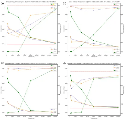
Figure 2: Cross-entropy in nats per character and frequency of sampling motif, depending on|D|. Two-stage Training. Features d0, d1, d2, d3 are on for all panels (f t[4:7] = {1111}). Panel (a): pureD, featuresm+0 (super-motif) andm/2 (sub-motif) on; (b): pureD,m(motif) andm/2(sub-motif) on; (c) pure D,mon; (d) mixtureD,mon. The plain lines represent cross-entropy, the dashed lines motif frequency.
the process for generating the training data. By contrast, the four remaining features are “distrac-tors”: d0 = 0iffxbegins with a0,d1 = 0 (resp.
d2 = 0,d3 = 0) iff a certain random, but fixed,
string of similar length tom(resp. of larger length, of smaller length) appears inx. We test different configurations of these features for training , and document the use/non-use of features with a bit-vectorf tof length|F|, for instancef t= 0111111 means that all features are exploited, apart from m.3
3In the experiments reported here, one of the provided features,m, is a detector of the motif actually present in the
data generating process, an extreme form of prior knowledge used to illustrate the technique. In general, milder forms of useful prior features can be provided. A simple formal exam-ple is to consider one real-valued (non binary) feature for the length, and one for the square of the length, an experiment
7.3 Implementation aspects 7.3.1 Autoregressive models
The AMs are implemented in PyTorch4 (Paszke
et al.,2017) using a 2-layered LSTM (Hochreiter and Schmidhuber, 1997) with hidden-state size 200. The input is presented through one-hot en-codings over the vocabularyV = {0,1,hEOSi}. These LSTMs are optimized with Adam (Kingma and Ba,2014), with learning rate↵ = 0.001, and that we did recently but do not report here; by matching the data expectations of these two additional features, the model is able to represent the mean and variance of length in the data. Here the prior knowledge provided to the model just tells it to be attentive to the distribution of length, a much weaker form of prior knowledge than telling it to be attentive to a specific motif.
4
[image:6.595.84.500.61.459.2]with early stopping (patience= 20) over a valida-tion set.
7.3.2 Training: Two-Stage and Cyclical The implementation is described in (Algorithm1). Here we provide some additional details.
Training-1 For training P (x) we test two regimes in Eq. 5, namely rs and snis; in both cases, we first train r(x) on the whatever D is available, and use it as the proposal distribution. During rs, we compute the model’s expectation over 10 accepted samples, update the ’s accord-ing to (5), and iterate. During snis, we keep a buffer of the last 5 ·104 samples from r(x) to compute the weighted average of the feature mo-ments. For the training of ’s, we use a basic SGD optimization with learning rate↵(#epoch) =
↵0
1+#epoch,↵0 = 10. To assess the quality ofP (x)
for early stopping during training, we use the dis-tance between the empirical and model moments:
`1 mom =
1
|D| X
d2D
(d) Ex⇠p (·) (x)
1
. (6)
Training-2 and Cyclical Training When dis-tilling from P in Training-2, we use a single proposalr, and systematically produce a distilled dataset of size DsSize = 2 ·104, which
corre-sponds to the highest value of |D| among those considered for trainingr. In Cyclical Training, the distillation process is performed in several stages, with an evolvingrfor improving the rejection rate.
8 Results
8.1 Cross-entropy comparison
We conduct experiments to compare the cross-entropy (measured in nats) between the initial AM r(x) relative to the test set T and the final AM ⇡✓(x) also relative to T; we vary the size of |D|2{0.5,1,5,10,20} ·103, the regimes (tReg) for Training-1 (rsorsnis), the features employed, the rarity of the motifs. Figure 2 depicts the re-sulting curves at the end of the two-stage training (plain lines).
Here we show only a few experiments (a more extensive set is provided in the [SM]).
We observe that, for a small dataset size |D|, there is a big gap between the CE of r(x) and the CE of ⇡✓(x). As|D|increases, these
cross-entropies become closer to one another, but a large gap persists for|D|= 5000.
We note that the presence of the “fully-predictive” feature m results in a ⇡✓(x) that has
CE very close to the theoretical entropy, even in low|D|regimes, whereron its own is very weak.5
Thus, not only is the distilled AM much better than the initial AM, but this is an indication thatP it-self (for which the cross-entropy is more difficult to compute exactly) is a good approximation of the true process.
By contrast, if the m feature is absent, then, while⇡✓ is still better thanr in low|D|regimes,
it cannot reach the theoretical entropy in such regimes, because features such as m0+ andm/2
can only partially model the data. With large|D|, on the other hand, r on itself does a good job at predicting the data, andP adds little on top of its rcomponent.
Finally, we note that the two regimes for train-ingP (x),rsandsnis, result in⇡✓’s with similar
accuracies.
We also observe that with a good performance of⇡✓(x), the moments of motif feature on the
dis-tilled dataset are close to the true ones (see [SM] Figure4,5,7).
These trends are consistent across the experi-ments with different motifs, as can be checked in Table3and with the additional plots in the [SM].
8.2 Motif frequencies
In order to assess the predictive properties of obtained AMs, we also compare the frequency of motifs in strings sampled from r and from ⇡✓ (2 · 103 samples in total). From Figure 2
we see that when vary |D|, the frequency of motifs (dashed lines) is aligned with the CE performance. Namely, ⇡✓ produces a higher
fraction of strings with motif than r when |D|is small (|D|2{0.5,1,5} ·103).
Detailed illustrationTo provide more intuition, we provide an illustration from one experiment in Table1.
8.3 MixtureDmamvs pureDm
In our experiments, the strings in Dmam (motif-anti-motif) contain a motif withp = 0.9. How-ever, if not all of the samples inDmamcontain the
1 true 101100010111110001000001001001
2 r 011111000010111110001110001011
3 ⇡✓ 111010100010111110000111111100
4 f t [m, , , d0, d1, d2, d3]
5 ’s [ 10.1, , , 0.15, 0.06,0.0, 0.14]
6 momtrue [0.0, , ,0.47,0.99,1.0,0.91] 7 momr [0.95, , ,0.53,0.99,1.0,0.91] 8 mom⇡✓ [0.0006, , ,0.43,0.99,0.99,0.91]
9 CEs true: 0.45,r: 0.56,⇡✓: 0.47
[image:8.595.173.430.59.199.2]10 motif freqs true: 1.0,r: 0.045,⇡✓: 0.959
Table 1: Illustration. Setting is from Fig. 2, panel (c): n =30, motif = 10001011111000 (always present inD), ft = 1001111, |D| = 5000, rs used for Training-1. Lines 1,2,3 show one example fromtrue, r,⇡✓ respectively;
with training set of size 5000,ris only able to generate the motif a fraction of the time (0.045, see line 10), but is better able to generate some submotifs (underlined);⇡✓generates the motif frequently (0.959), as illustrated on
line 3. With the features fromf t(line 4), Training-1 produces aP with first feature mstrongly negative (line 5),
meaning thatP strongly penalizes the absence of the motif; the “distractor” featuresd0, d1, d2, d3 get a weight close to0, meaning that they have little predictive power in combination with featurem. It is visible from lines 6,7,8 that⇡✓ is much better able to approximate the true feature expectations thanr[features expectations (aka
moments) underr(resp.⇡✓) : Ex⇠r(·) (x)(resp.Ex⇠⇡✓(·) (x)) ] Finally (line 9), the CE of⇡✓relative to the
test set is close to the true entropy of the process, while that ofris much further away.
|D| m; mtf frqrs mtf frqsnis m;
CE(rs)
CE(snis) m;
time(rs)
time(snis) mam;
mtf frqrs
mtf frqsnis mam; CE(rs)
CE(snis) mam;
time(rs)
time(snis)
500 0.998 0.967 2.92 0.997 1.003 4.7
1000 1.009 0.973 2.038 0.77 1.07 3.638
5000 0.995 0.967 0.756 1.12 0.99 1.365
10000 1.134 0.956 1.514 1.011 1.002 1.005
20000 1.497 0.961 0.938 0.965 1.005 0.975
Table 2: Comparison of the time for Training-1 inrs andsnis; for motif 10001011111000; f t = 1011111; H(ptrue) = 0.449with pureD (m) andf t = 1001111; H(ptrue) = 0.482with mixture of motif-anti-motifD
(mam).
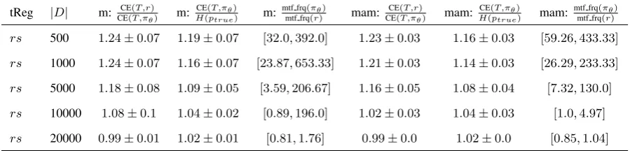
tReg |D| m: CE(T,r)
CE(T,⇡✓) m:
CE(T,⇡✓) H(ptrue) m:
mtf frq(⇡✓)
mtf frq(r) mam:
CE(T,r)
CE(T,⇡✓) mam:
CE(T,⇡✓)
H(ptrue) mam:
mtf frq(⇡✓)
mtf frq(r)
rs 500 1.24±0.07 1.19±0.07 [32.0,392.0] 1.23±0.03 1.16±0.03 [59.26,433.33]
rs 1000 1.24±0.07 1.16±0.07 [23.87,653.33] 1.21±0.03 1.14±0.03 [26.29,233.33]
rs 5000 1.18±0.08 1.09±0.05 [3.59,206.67] 1.16±0.05 1.08±0.04 [7.32,130.0]
rs 10000 1.08±0.1 1.04±0.02 [0.89,196.0] 1.02±0.03 1.04±0.03 [1.0,4.97]
rs 20000 0.99±0.01 1.02±0.01 [0.81,1.76] 0.99±0.0 1.02±0.0 [0.85,1.04]
Table 3: Overall statistics: forDm, motif 2{10001010001,01011101101,001001100111,1011100111001,
10001011111000}, f t 2 {1001111,1011111,0111111} and Dmam, motif 2
{01011101101,001001100111,1011100111001,100010100011,10001011111000},f t2{1001111}.
motif, then the motif feature itself is not fully pre-dictive. It can be seen in panel (d) of Figure2that the⇡✓achieved withP trained on mixtureDmam
[image:8.595.75.525.335.468.2] [image:8.595.74.524.533.641.2]8.4 Regimes in Training-1
For training GAM we consider two methods,snis andrs. As described in the previous sections, their impact onP leads to⇡✓’s that have similar CE’s
and motif frequencies. Despite such resemblance in terms of accuracy, these two methods differ in terms of speed (see Table2). Namely, whenr is close to white noise due to small|D|, then for the rare eventsrsrejects most samples not containing the motif due to the effect of the log linear term and negative value of the component m corre-sponding to the m feature, while snis is able to exploit all samples. Despite being faster thanrs, snisremains competitive in terms of CE.
8.5 Cyclical vs two-stage training
We conducted a small experiment to compare the performance of cyclical training with two-stage training in terms of speed and accuracy for a fixed motif m and featuresf t (see [SM] Table4, Fig-ure3). We observed that CEs of the obtained⇡✓’s
were about the same for different values of|D|and Training-1 regimes. On the other hand, there was no systematic improvement in the training speed of one method over the other.
9 Discussion
The basic idea behind GAMs is very simple. First, we extend the representational power of the au-toregressive model r by multiplying by a log-linear potential, obtaining an unnormalized model P (Training-1). Then we try to “project” this ex-tended representation again to an autoregressive model ⇡✓ (Training-2). Our results showed that,
under favorable prior knowledge conditions, the fi-nal⇡✓ was able to perform as well, when trained
on small data, as the standard r, trained on large data. During our experiments, we noticed that training P was actually easier than training ⇡✓
from it. Intuitively, the small number of param-eters to be fitted in the log-linear model requires less work and fewer data than the training of an autoregressive component.6
6At a deeper level, there are extreme situations where the
P obtained at the end of Training-1 can perfectly represent
the true process, but where no autoregressive model can ac-tually fitP : one way to obtain such situations consists in
generating binary strings that satisfy a certain cryptographic predicate, associated with a specific feature; the importance of this feature can be easily detected through Training-1, but an autoregressive model has no chance of generalizing from distilled or true data, even in large quantities.
It is interesting to relate our study to certain as-pects of Reinforcement Learning (RL).
First, consider Training-2. There, we have a “score” P that we are trying to approximate through an autoregressive model⇡✓, which is
ba-sically a sequential “policy”. The main difference with RL is that we are not trying to find a policy thatmaximizes the score (which would be a bad idea for language modelling, as it would tend to concentrate the mass on a few sequences), but one that approximatesP in adistributionalsense; our current distillation technique is only one way to approach this problem, but other techniques more in the spirit of RL are possible, a direction that we leave for future work.
Second, consider Training-1. Our approach, consisting in suggesting to the model a number of prior features, might look too easy and suspicious. But notice that in RL, one would typically directly provide to the model an externally definedreward, a very strong form of prior knowledge. Here, in-stead, we “only” indicate to the models which fea-tures it might attend to, and Training-1 then deter-mines the “reward”P through max-likelihood, a milder form of prior knowledge, more respectful for what the data has to say.7
Acknowledgements
Thanks to Matthias Gall´e and Ioan Calapodescu for com-ments on a previous version of this paper and to the anony-mous reviewers for their detailed reading and feedback.
References
Daniel Andor, Chris Alberti, David Weiss, Aliaksei Severyn, Alessandro Presta, Kuzman Ganchev, Slav Petrov, and Michael Collins. 2016. Globally Nor-malized Transition-Based Neural Networks.
Marc G. Bellemare, Will Dabney, and R´emi Munos. 2017. A Distributional Perspective on Rein-forcement Learning. arXiv:1707.06887 [cs, stat]. ArXiv: 1707.06887.
Rafael C. Carrasco. 1997. Accurate computation of the relative entropy between stochastic regular gram-mars. Theoretical Informatics and Applications, 31:437–444.
Corinna Cortes, Mehryar Mohri, Ashish Rastogi, and Michael Riley. 2008. On the computation of the relative entropy of probabilistic automata. Int. J. Found. Comput. Sci., 19(1):219–242.
Jonas Gehring, Michael Auli, David Grangier, De-nis Yarats, and Yann N. Dauphin. 2017. Convolu-tional sequence to sequence learning. CoRR. Cite arxiv:1705.03122.
Geoffrey E. Hinton, Oriol Vinyals, and Jeffrey Dean. 2015. Distilling the knowledge in a neural network. CoRR, abs/1503.02531.
Cong Duy Vu Hoang, Ioan Calapodescu, and Marc Dymetman. 2018. Moment Matching Training for Neural Machine Translation: A Preliminary Study.
Sepp Hochreiter and J¨urgen Schmidhuber. 1997. Long short-term memory. Neural computation, 9(8):1735–1780.
Tony Jebara. 2013. Log-Linear Models, Logistic Re-gression and Conditional Random Fields.
Michael I. Jordan. 2010. Chapter 8 The exponential family : Basics.
Diederik P Kingma and Jimmy Ba. 2014. Adam: A method for stochastic optimization. arXiv preprint arXiv:1412.6980.
Yann LeCun, Sumit Chopra, Raia Hadsell, Marc’Aurelio Ranzato, and Fu Jie Huang. 2006. A Tutorial on Energy-Based Learning. Predicting Structured Data, pages 191–246.
Andrew Y. Ng and Stuart J. Russell. 2000.Algorithms for inverse reinforcement learning. InProceedings of the Seventeenth International Conference on Ma-chine Learning, ICML ’00, pages 663–670, San Francisco, CA, USA. Morgan Kaufmann Publishers Inc.
Art Owen. 2017. Adaptive Importance Sampling (slides).
Adam Paszke, Sam Gross, Soumith Chintala, Gre-gory Chanan, Edward Yang, Zachary DeVito, Zem-ing Lin, Alban Desmaison, Luca Antiga, and Adam Lerer. 2017. Automatic differentiation in PyTorch. InNIPS Autodiff Workshop.
Christian P. Robert and George Casella. 2005. Monte Carlo Statistical Methods (Springer Texts in Statis-tics). Springer-Verlag, Berlin, Heidelberg.
Stuart Russell. 1998.Learning agents for uncertain en-vironments (extended abstract). InProceedings of the Eleventh Annual Conference on Computational Learning Theory, COLT’ 98, pages 101–103, New York, NY, USA. ACM.
Ilya Sutskever, Oriol Vinyals, and Quoc V. Le. 2014.
Sequence to sequence learning with neural net-works. InAdvances in Neural Information Process-ing Systems 27: Annual Conference on Neural In-formation Processing Systems 2014, December 8-13 2014, Montreal, Quebec, Canada, pages 3104– 3112.
Richard S. Sutton and Andrew G. Barto. 2018. Rein-forcement Learning: An Introduction, second edi-tion. The MIT Press.
Ashish Vaswani, Noam Shazeer, Niki Parmar, Jakob Uszkoreit, Llion Jones, Aidan N. Gomez, Lukasz Kaiser, and Illia Polosukhin. 2017. Attention is all you need. InAdvances in Neural Information Pro-cessing Systems 30: Annual Conference on Neural Information Processing Systems 2017, 4-9 Decem-ber 2017, Long Beach, CA, USA, pages 6000–6010.