Abstract—Fault detection is essential for the survivability of many systems. Since many systems present highly nonlinear dynamics, the applicability of general fault detection techniques designed mainly for linear systems is very questionable. In this communication, after introducing the concept of difference flat nonlinear systems, a fault detection scheme based on difference flatness is proposed.
Index Terms—Fault detection, differential flatness,
rotorcraft.
I. INTRODUCTION
In the last decade a large amount of interest has risen for new fault detection and identification (FDI) approaches for non linear systems. However few results have been obtained through purely non linear approaches. Differential flatness, a property of some nonlinear dynamic systems, introduced by Fliess et al. from the theory of differential geometry, has made possible the development of new tools to control effectively nonlinear systems. Many dynamic non linear systems have been proved to be differentially flat and the differential flatness of conventional and non conventional aircraft dynamics has been proven in different situations. While there are many different approaches to cope with fault detection in the case of linear systems, this is not the case with non linear systems and in this paper we introduce a fault detection technique applicable to difference flat non linear systems.
In the first part of this paper, the main concepts relative to difference flatness applied to discrete dynamical systems are particularly considered. Then a new approach, based on the redundancy between flat outputs and direct state component measurements, is proposed. To take into account measurement errors as well as modelling errors to perform fault detection tests in this non linear context, probabilistic distributions are generated on-line. However the resulting distribution for the state estimates of a nonlinear system will
N. Zhang is with Laboratoire d’Architecture et d’Analyse des Systèmes-CNRS, Toulouse, France, [email protected].
A. Doncescu is with Laboratoire d’Architecture et d’Analyse des Systèmes, CNRS, Toulouse, France, [email protected].
A.C. Brandão Ramos is with UNIFEI, Itajuba, Brazil, , [email protected] F. Mora-Camino (corresponding author) is with LAAS du CNRS and Automation and Operations Research Laboratory at the Air Transportation Department of the French Civil Aviation Institute-ENAC, Toulouse, France, [email protected], Tel. 0033562174358, fax 0033562174403.
Fault Detection for Difference Flat Systems
Nan Zhang , Andrei Doncescu, Alexandre C. Brandão Ramos and Felix Mora-Camino
not be Gaussian in general and its full construction should need intensive computation which is not affordable in an online context. So, from a reduced set of distributions points a fuzzy membership function is constructed and a comparison, through a reduced number of fuzzy logic rules can be performed to get a fault diagnostic. The proposed scheme is illustrated in the case of a rotorcraft subject to faults characterized by parameter shifts.
II. DIFFERENCE FLAT SYSTEMS A. Difference flat systems of order (p,q)
Consider a non-linear system whose discrete time dynamics are given from an initial state X0 by:
(
k k kk X f X U
X +1= + ,
)
(1) for k∈N, where nk R
X ∈ , m
k R
U ∈ , is a smooth vector field of
f
k
X
and Uk which are respectively the state and the input vectors of this system at time k. It is supposed here that each input has an independent effect on the state dynamics:{
mj i with j i u f u
f ∂ i ≠∂ ∂ j, ≠ , , ∈ 1,...,
}
∂ (2)
The system given by (1) is said to be difference flat of order (p,q), where p and q are integers, if there exists a measurable output
Y
∈
R
m:(
kk h X
Y =
)
(3) whereh
is a smooth vector field of Xk , such as it is possible to write:(
k p k p k q)
k Y Y Y
X =η + , + −1,..., − (4)
(
k p k p k q)
k Y Y Y
U =ξ + +1, + ,..., − (5) where η
( )
. is a function ofY
j and its values fromback to order
j
p
k
+
j
q
k− , and that ξ
()
. is a function of Yj and itsvalues from k+pj+1 back to k−qj, for j = 1 to m.
Here p and q are given by:
{ }
j tomj p
p
1 max
=
= and
{ }
j tom
j q
q
1
max =
= (6) For j=1 to , is called the discrete relative degree of output
m pj
j
Y , while pj+qj is the time span of the dynamics of output j. It is easy to show that:
(
)
∑
=
≤ +
m
j
j
j q n
p
1
` (7) B. Nominal state reconstruction
steps:
- At current time, the set of measurements
)
,
,
,
,
(
Y
k−qY
k−q+1L
Y
k+p−1Y
k+p is available, so it ispossible when the model of the discrete dynamics and the measurements are assumed to be perfect, to compute the exact value of the state of the system at time k by the discrete flat relation:
(
1,..., 1~
q k p k
k Y Y
X =η + −
)
(8) - Then, starting from this value and using repeatedly the discrete state equation (1) from time to timewith the past known inputs U
k h=
1 − + p
k h :
(
h h)
h
h X f X U
X~ +1= ~ + ~ , (9)
we get the current state valueX~k+p.
Unfortunately, discretized models and measurements present in general systematic errors and the above scheme cannot be used directly.
III. THE PROPOSED FAULT DETECTION SCHEME
The proposed detection scheme is based on the redundancy of information which is present when considering simultaneously flat outputs and some state components of a system subject to faults. So, here we consider that an output composed of a flat output vector and p additional components of the state vector is available at each time period:
⎥ ⎦ ⎤ ⎢ ⎣ ⎡ +
⎥ ⎥ ⎥ ⎥ ⎥
⎦ ⎤
⎢ ⎢ ⎢ ⎢ ⎢
⎣ ⎡
=
⎥ ⎥ ⎥ ⎥ ⎥
⎦ ⎤
⎢ ⎢ ⎢ ⎢ ⎢
⎣ ⎡
=
k k
i i k
i i k
k
v
x x Y
x x Y
Z
r r
υ μ
μ μ
M M
1
1 (10)
with m+r≤n where m
k R
v ∈ and r
k∈R
υ are
measurements errors.
Since in theory it is possible to reconstruct the state of the system from past and present flat outputs and inputs, at current time it will be possible to compute residuals such as:
p k+
j
j i
i p k
j X X
X ,+ = μ− ~
δ j=1 to r (11) and considering the accuracy of the measurement channels and of the discretized model, it should be possible to set thresholds to detect faults in the system. Then the satisfaction of tests such as:
p j
X
j , =1,L,
σ
{
}
Xj p k j
X r j
if ∃ ∈ 1,L, :δ , + >σ (12)
will indicate the presence of a fault with some probability
{
r
}
j
j
,
∈
1
,
L
,
π
.Of course, the effectiveness of this fault detection scheme is directly dependant of the levels of these thresholds. To investigate this point, additional assumptions are made here: It is supposed that the measurement error follow Gaussian white noise processes with zero means:
{ }
vk =0E (13) and with constant variances given by:
{ }
{
i}
kht h
k v diag V i tom
v
E ,
2 1
, = δ
= (14)
where δk,h=0if k≠handδk,k=1 (15) In the same way, we suppose that:
E
{ }
υ
k =0 (16) and
{
t}
{
i}
khh
k diag i to p
E ,
2 1
, δ
υ
υ = Δ = (17)
where δk,h=0if k≠handδk,k =1 (18) The modeling error can be also approximated by additive gaussian white noises such that the state dynamics of the system under consideration can be rewritten:
k k k k
k X f X U
X +1= + ( , )+ω (19) where
ω
k is a Gaussian white noise vector of dimension nsuch as:
{ }
k =0Eω (20)
and E
{
k ht}
diag{
Wi i ton}
k,h 21
, δ
ω
ω = = (21)
To define the appropriate probability levels used in the fault detection test, since the flatness relation and the state equation are in general non-linear, the probability distribution of the estimation errors through the reconstruction process described in subsection II.B does not follow necessarily a Gaussian distribution. Then, it is necessary to generate on line the probability distribution of the error of the current state estimations.
IV. GENERATION OF STATE DISTRIBUTIONS
It is possible to generate, using the process described above through different realizations of the modeling and measurement errors, statistics for the estimates at current time k+p of the state of the difference flat system. The generation process for state distribution at period k+p if composed of two stages: random generation of the state distribution at period k, through flat differential equation, and then random generation of state distribution at period k+p through state equation propagation from period k to period k+p.
We get first estimates at time k, ( , , ) q p i
i
k
X
−
L
)
, where the vectors of indexes
i
h are such as:{
p p q}
h N
ih∈ m, ∈ , −1,L,− (22) Then we get:
) , , ( ) , ,
(p q p iq
q k i
p k i
i h
k Y Y
X
− −
− +
− = L
) L
η
(23) For each choice s of
i
h,i
hj,s the flat output component,m to
j=1 , present in η is computed according to:
}
{
q p
p h
N N i
V i Y
Y j hjs
s h j h k j i
h j
h j
− − =
− ∈ ⋅
+
= +
, , 1 ,
, , , ,
, , ,
L
L μ
(24)
Let ihjs be the associated probability given by:
h j
,
, ρ
N to N i V i
j h j i
h j
s h
j =−
⋅ − =
π ρ
2 )
exp( 2
,
,
(25) Let be the maximum number of different estimates which is generated according to relations 29 and 30 at time k+p for each component of the state of the difference flat
max
s
ISBN: 978-988-19251-9-0
ISSN: 2078-0958 (Print); ISSN: 2078-0966 (Online)
system at time k.
s
max is such as:) 1 ( max (2 1)
+ + ⋅ +
≤ N m p q
s (26) Since this number can be excessive (for N= 5, m =3, p =2, q =1 we get ), the number of choices for s must be strongly limited. For a single choice of s among
, we generate for N = 5, m = 3, p =2 and q =1, s 12
max ≈3.10 s
}
{
−N,L,N max= 12 different values for each state component and then smax=
4090 different values when two different choices are done for s. By similarity with the particular filtering approach, we will
call particle each generated state ( , , ) q p i
i
k
X
−
L
)
for time k from measurements
Y
μk−q toμ
p k
Y
+ . Letr
k
X
ˆ
be the estimate of the state for period k generated at period k+p,th
s
1
=
s
to .max
s
For each particle, following (25), we get for the next periods until current time (h = k to k+p-1) the following r.
n
maxstate estimates:) , , ( ( , , ) )
, , ( ) , , , (
1
1 k h h h h
h h
k r
h h r r h r
r h r r r
h X f X U
X( +L + = ( L + ( L ω(
with
s
h 1s
maxh (27)max
=
2
⋅
+
for sh =1 to , with the initial conditions: h
s
maxmax max max
) (
1
ˆ forr tos with s s
X
X r k k
k r
k
k = = =
(
(28) where sh
h
ω
(
is a random try for the Gaussian vectorω
h towhich is associated the probability:
∏
= ⎟⎟⎠
⎞ ⎜⎜
⎝ ⎛
− ⋅ ⋅
= n
s
s r
h s s
s
h W
W
1
2 , / ) /2
( exp 2
1 ω
π
α ( (29)
Then, with the chosen generation process, we get different estimates of the current state of difference flat system. Each of this estimates are characterized by the vectors of indexes such as:
max 2rs
(
r ,r 1, ,r)
withs{
1, ,2 smax}
k h h
p k k k
− +
+ L ∈ L (30)
Let the weights (sk, ,sk p) be given by:
p k j
P
++L
) (
/ )
( ,, ,,
) , , (
∏
∑
∑
∏
+− = +
− =
+ = ⋅ ⋅
+ − +
p k
q k h
s h i
h j s
s p
k
q k h
s h i
h j s
s p k j
h s h j p
k q k h s h j p
k k
P L ρ α L ρ α (31)
It is then possible to compute approximations of the first and second order statistics for each measured state component at current time:
) ( ( , , ) (k, ,k p) q
k
p k k
p k
s s
p k s
s s
p k s p
k P X
X +
−
+
+
+ +
+ =
∑ ∑
L L (
L (32)
with an estimate of the standard deviation of
X
~
jk+p given by:2 )
, , ( ) , , (
) (
( ~
p k j s s
p k j s
s s
p k s p
k
j P X X
V k k p
q k
p k k p k
+ +
+
+ = + −
−
+ +
∑ ∑
L LL (33)
V. THE FAULT DETECTION SCHEME A. Building a fuzzy estimation
From the above generation it is now possible to build a fuzzy representation for each measured component of the
state vector. Considering for each component i of the state vector the set of points ( (sk, ,sk p) ,
p k
P +
+ L Xi(ksk,p ,sk p)
+
+L
( ), a
membership function can be taken as a scaled polynomial interpolation of this set of points when the current state component is taken as the independent variable (see figure 1). Only the positive part of the polynomial interpolation will be retained, this ensures that its base
) (x ajk+p
0 p k j
B
(
+ which is the smallest convex covering set of{
( ) 0}
0 = >
+
+ xa x
Bjk p jk p , is finite : +∞ < + 0
p k j
[image:3.595.305.548.63.405.2]B( (34)
Figure 1: generated membership function
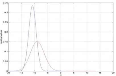
Figure 2-Comparison of measure and estimate distributions.
Then the membership function for
x
j(
k
+
p
)
is given by:{
( )}
max / ) ( )
(x a x ajk p y
R y p k j p k
j + = + ∈ +
μ for j =1 to r (35)
It is also possible to consider a Gaussian distribution for
p k j
X
~
+ given by:)) ~ 2 /( ) (
exp( ~ 2
1 ) (
~ 2
p k j p k j
p k j p
k
j x X V
V x
f + +
+
+ = − −
π
(36)
B. Measuring the difference between estimates
The discrepancy between the distribution of and the Gaussian distribution is computed by:
p k j
X
, +) )) ( ~ ) ( ( ( ~ 2
1 2
dx x f x a V
Qjk p jk p
∫
jk p jk p+∞
∞ −
+ + +
+ = − π −
for j =1 to r (37) so that if the generated distribution is similar with a Gaussian distribution while if is near to zero or negative, the generated distribution is quite different from a
1
= +p k j
Q
p k j
[image:3.595.321.525.361.494.2]Gaussian distribution. This parameter is important because according with the degree of similarity with a Gaussian distribution, the comparison with the measurement data will be performed differently since to the measurement is associated another Gaussian distribution whose standard deviation factor is directly related with the accuracy of the measurement device:
)) 2 /( ) (
exp( 2
1 )
( 2
j p k j
j p
k
j x x X
f − − Δ
Δ
= +
+ μ
π
(38)
Normalization of this distribution provides a membership function
f
jk+pfor the measure of Xj at time k+p:)) 2 /( ) (
exp( )
( jk p 2 j
p k
j x x X
f + = − − μ+ Δ (39)
Then, the detection of faults which here is based on a discrepancy between the measurement and the estimation of can be performed by comparing their membership functions, see figure 3. Then it is possible to compute a membership function for the intersection of the corresponding fuzzy sets by:
p k j
X
, +) ( ~ ) ( )
(x x f x
[image:4.595.318.533.58.163.2]wjk+p =μjk+p jk+p
x
∈
R, for j=1 to p (40)Figure 3. Comparison of a Gaussian and a general membership functions
which can be characterized, if it not identically null, by the following parameters.
Its mean value:
dx x w dx x x w X
p k j p
k
j B
p k j B
p k j w
p k
j
∫
( ) /∫
( )+ +
+ +
+ = (41)
Its maximum value: max max ( ) (42) x w
X jk p
B x w
p k j
p k j
+ ∈
+
+ =
Its base ratio :
b
wjk+p=
B
(
wjk0+p/
B
(
j0k+p (43) where is the minimum convex covering set ofgiven by: 0
w p k j
B( +
0 w
p k j
B
+ 0 ={
>0}
+
+ jk p
w p k
j x w
B (44)
Its medium cut set ratio:
0 5 . 0
/ wjk p w
p k j w
p k
j + = B + B +
( (
τ (45)
where is the minimum convex covering set of given by:
5 . 0
w p k j
B + (
5 . 0
w p k j
B +
{
}
⎭ ⎬ ⎫ ⎩
⎨
⎧ ∈ >
= + +
+.5 ( ) 0.5max ( )
0
y w x
w R x
B jk p
y p
k j w
p k
j (46)
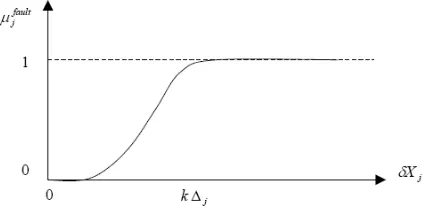
Given for state component j a typical fault diagnosis curve such as:
Figure 4. Fault membership function for state component j
C. Computation of the more likely discrepency
It is then possible using a set of practical rules based on parameters Xμjk+p,Δj,Xjk+p,Vjk+p, ,
~
p k j
Q + Xwjk+p, ,
and , to compute the more likely discrepancy between the measurement of Xj and its estimate at current time k+p. For instance when:
max
w p k j
X +
w p k j
b + τwjk+p
p k j
X
ˆ
+δ
1
≈ +p k j
Q then
δ
Xˆjk+p ≈ Xjk+p −Xμjk+p (47)and when:
0
≈ +p k j
Q then
δ
w μjk p (48)p k j p k
j X X
Xˆ + ≈ max+ − +
Then considering all the state components at current time k+p, the likelihood of a fault at current time k+p will be given by:
{
( ˆ )}
max
1 jk p
fault j r to j fault
p
k+ = = μ δX +
μ (49)
with a fault generalization degree given by:
{
( ˆ )}
min
1 jk p
fault j r to j fault
p
k+ = = μ δX +
μ (50)
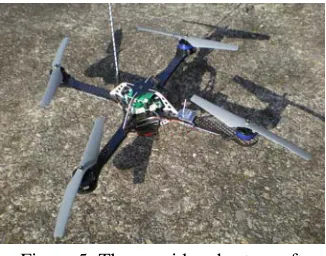
VI. APPLICATION TO A ROTORCRAFT
The considered system is shown in figure 5 where rotors one and three are clockwise while rotors two and four are counter clockwise. The main simplifying assumptions adopted with respect to flight dynamics in this study are a rigid cross structure, constant wind, negligible aerodynamic contributions resulting from translational speed, no ground effect as well as small air density effects and negligible response times for the rotors.
A. Rotorcraft dynamics
The rotor forces and moments are given by: 2
i i f
F = ω i∈
{
1,2,3,4}
}
(51-1)
2
i i
i kF k f
M = = ω i∈
{
1,2,3,4(51-2)
ISBN: 978-988-19251-9-0
ISSN: 2078-0958 (Print); ISSN: 2078-0966 (Online)
[image:4.595.61.283.311.462.2]Figure 5: The considered rotorcraft
Where f and k are positive constants and ωi is the rotational speed of rotor i. These speeds and forces satisfy the constraints:
max
0≤ω ≤ω i
i i∈
{
1,2,3,4}
(52-1)}
{
1,2,3,40≤Fi ≤Fimax= f max i∈
i ω
(52-2)
Since the inertia matrix of the rotorcraft can be considered diagonal with Ixx = Iyy, the roll, pitch and yaw moment
equations may be written as:
xx I r q k F F l
p& =( ( 4− 2)+ 2 )/ (53-1)
q&=(l(F1−F3)+k4pr)/Iyy (53-2) r&=(k(F2−F1+F4−F3))/Izz (53-3)
where p, q and r are the roll, pitch and yaw body angular rates. Here k2=(Izz−Iyy) and k4=(Ixx−Izz), where Ixx, Iyy and Izz are the inertia moments in body-axis, and l is the
length of the four arms of the rotorcraft.
Let φ, θ and ψ be respectively the bank, pitch and heading angles, then the Euler equations relating the derivatives of the attitude angles to the body angular rates, are given by:
) cos )(sin
( q r
tg
p θ φ φ
φ&= + + (54-1)
r
q φ
φ
θ&=cos −sin (54-2)
θ φ
φ
ψ&=(sin q+cos r)/cos (54-3)
In this study the wind is given in the local Earth reference frame by w=
(
wx wy wz)
' . The wind is supposed constant while the ground effects are neglected. Since the rotorcraft operates at low speeds, the drag can be neglected. Then the acceleration a=(
ax ay az)
' of the centre of gravity, taken directly in the local Earth reference frame is given by: ) )) sin( ) sin( ) cos( ) sin( ) )((cos( / 1( m F
ax= ψ θ φ + ψ φ (55-1)
) )) sin( ) cos( ) cos( ) sin( ) )((sin( / 1
( m F
ay= ψ θ φ − ψ φ (55-2)
) ) cos( ) )(cos( / 1
( m F
g
az = − θ φ (55-3) where x, y and z are the centre of gravity coordinates, m is the total mass of the rotorcraft and:
(56) 4
3 2
1 F F F
F
F= + + +
In equations (47-1) and (47-2), the effects of the rotor forces appear as differences so, we define new attitude inputs uq and up as:
3 1 F
F
uq= − up=F4−F2 (57) In the heading and position dynamics, the effects of rotor forces and moments appear as sums, so we define new guidance inputs uψand uz as:
) ( )
(F2 F4 F1 F3
uψ = + − + uz=F=F1+F2+F3+F4 (58)
' ] [up uq u uz
u= ψ (59) Equations (47-1), (47-2) and (47-3) are rewritten:
xx
p k qr I
u l
p& =( + 2 )/ (60-1)
yy
q k pr I
u l
q&=( + 4 )/ (60-2)
zz I u k
r&= ψ / (60-3) B. Rotorcraft Discretized Dynamics
Adopting a first order discretization of the rotorcraft
dynamics with a time step δ, we get the discrete rotorcraft flight dynamics model:
( ) ( ) ( ) ( ) ( ) ( ) ( ) ( ) ( ) ( ) ( ) ( ( ) ( )) ( )
(
)
(
)
(
)
( ) ( ) ( )( ( ) ( ) ( ) ( ) ( )) ( ) ( )( ( ) ( ) ( ) ( ) ( )) ( ) ( ) ( ) ( ) ( ) ⎪ ⎪ ⎪ ⎪ ⎪ ⎪ ⎩ ⎪⎪ ⎪ ⎪ ⎪ ⎪ ⎨ ⎧ ⋅ ⋅ ⋅ + − ⋅ + = ⋅ ⋅ − ⋅ ⋅ ⋅ ⋅ + = ⋅ ⋅ + ⋅ ⋅ ⋅ ⋅ + = ⋅ ⋅ + = ⋅ ⋅ + ⋅ ⋅ + = ⋅ ⋅ + ⋅ ⋅ + = ⋅ + ⋅ ⋅ + = ⋅ − ⋅ ⋅ + = ⋅ ⋅ + ⋅ ⋅ + ⋅ + = + + + + + + + + + k t k k k k k t k k k k k k k k t k k k k k k k k r zz k k k k k q yy k k k k k p xx k k k k k k k k k k k k k k k k k k k k k k k k k u x x m g x x u x x x x x m x x u x x x x x m x x u I k x x x x k u I a x x x x k u I a x x x x x x x x x x x x x x x x x x x x x x x x x , , 1 , 2 , 9 1 , 9 , , 1 , 3 , 1 , 2 , 3 , 8 1 , 8 , , 1 , 3 , 1 , 2 , 3 , 7 1 , 7 , , 6 1 , 6 , 6 , 4 4 , , 5 1 , 5 , 6 , 5 2 , , 4 1 , 4 , 6 , 2 , 1 , 5 , 2 , 1 , 3 1 , 3 , 6 , 1 , 5 , 1 , 2 1 , 2 , 6 , 1 , 2 , 5 , 1 , 2 , 4 , 1 1 , 1 cos cos 1 sin cos cos sin sin 1 sin sin cos sin cos 1 cos cos cos sin sin cos cos tan sin tan δ δ δ δ δ δ δ δ δ (61)where the state vector Xk is given by:
[
]
′= k k k k k k k k k
k p q r x y z
X φ θ ψ & & & (62) where
φ
k is the bank angle, θk is the pitch angle,ψ
kis the heading direction, pk is the roll rate,qk is the pitch rate, rk isthe yaw rate , are the components of the rotorcraft translational speed in the Earth reference frame.
k k
k y z
x& ,& ,&
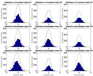
figure 6 displays the corresponding error histograms, showing that the Gaussian hypothesis for modeling is acceptable in the current case.
Here we have applied the state distribution generation method proposed in section 4.. It has been supposed that the nine components of the state of the discrete version rotorcraft are measured while the first component of this state is the flat output from which the other two state components can be reconstructed (here p = 1) for one period before current decision time. To generate an initial distribution using the flatness relations and take into account the errors present in the flat outputs measurements, two values have been chosen for each output randomly to activate relation (30), leading to
( ) 2 256
2m⋅p+q+1 = 8 = different initial estimates.
Then applying twice relation (33) we get at current time a state distribution of 256 X 2 = 512 samples. These 512 samples are generated on line at each discrete instant and allow to estimate probabilistic distributions so that a fault test can be performed by comparison with the direct measurements of x4(= p), x5(=q) and x6(=r).
[image:5.595.95.258.49.177.2]Figure 6. discretization error histograms
Figure 7. Distribution comparison for x5 = q with fault
at t = 0.06 sec, t = 0.12 sec
VII. CONCLUSION
This communication proposes a new approach to detect faults occurring in nonlinear systems whose discrete dynamics are differencially flat. The proposed approach has been illustrated in the case of a rotorcraft. The proposed approach can be improved in different ways: other distribution generation schemes could be considered easily and compared with the one adopted here while the generated distribution could be used directly in the fault detection tests avoiding the gaussian hypotesis which has been adopted here for sake of simplicity.
REFERENCES
[1] Paul M. Frank, “Fault Diagnosis in Dynamic System Using Analytical and Knowledge-base Redundancy – A Survey and Some New Results”, Universität-GH-Duisburg, pp. 459-474, 1990.
[2] Del Moral P, “Nonlinear filtering using random particules”, Journal of Theory and Probability Applications, vol.40, pp.690-701, 1996.
[3] D. Crisan and A. Doucet, “A survey on convergence results on particule filtering for practitionners”, IEEE Transactions on
Signal Processing, vol.50, pp.736-746, 2002.
[4] A. Kandel, “Fuzzy Mathematical Techniques with Applications”. Addison-Wesley Publishers Company. ISBN: 0-201-11752-5, 1986.
[5] F. Mora-Camino and K. Achaibou, “A fault tolerant scheme for flight control”,IFAC Symposium on intelligent components and instruments for control applications, Malaga, Spain, 1992.
[6] F. Mora-Camino and A. Achaibou, “A fuzzy approach for data sensor failure detection”, IFAC workshop, Terrassa, Universidade Politecnica de Catalunya, 1993.
[7] W. C. Lu, L. Duan, F. Mora-Camino, K. Achaibou, “Differential Flatness and Fault Detection in Flight Guidance Dynamics”, Safeprocess, August 2006, Beijing, China.
[8] N. Zhang, A. Drouin, A. Doncescu and F. Mora-Camino, “Differential flatness approach for Rotorcraft Fault Detection”, Chinese Control Conference, July 2008, Kunming, China.
ISBN: 978-988-19251-9-0
ISSN: 2078-0958 (Print); ISSN: 2078-0966 (Online)
[image:6.595.53.273.257.344.2]