OPTIMAL TRANSPORT METHODS
C.J. BUDD∗, R. D. RUSSELL†, AND E. WALSH‡
Abstract. The principles of mesh equidistribution and alignment play a fundamental role in the design of adaptive methods [32], and a metric tensorMand mesh metric are useful theoretical tools for understanding a method’s level of mesh alignment, or anisotropy. We consider a mesh redistribution method based on the Monge-Amp`ere equation [17],[9], [10], [8], [7], which combines equidistribution of a given scalar density function ρwith optimal transport. It does not involve explicit use of a metric tensorM, although such a tensor must exist for the method, and an interesting question to ask is whether or not the alignment produced by the metric gives an anisotropic mesh. For model problems with a linear feature and with a radially symmetric feature, we derive the exact form of the metricM, which involves expressions for its eigenvalues and eigenvectors. The eigenvectors are shown to be orthogonal and tangential to the feature, and the ratio of the eigenvalues (corresponding to the level of anisotropy) is shown to depend, both locally and globally, on the value ofρ=√detM
and the amount of curvature. We thereby demonstrate how the optimal transport method produces an anisotropic mesh along a given feature while equidistributing a suitably chosen scalar density function. Numerical results are given to verify these results and to demonstrate how the analysis is useful for problems involving more complex features, including for a non-trivial time dependant nonlinear PDE which evolves narrow and curved reaction fronts.
Key words. Alignment, Anisotropy, Mesh Adaptation, metric tensor, Monge-Amp`ere.
AMS subject classifications. 35J96, 65M50, 65N50
1. Introduction. Efficiently and accurately computing solutions to PDEs (par-tial differen(par-tial equations) which exhibit large variations in small regions of a physical domain frequently demands using some form of mesh adaptation/redistribution. It is often desirable to adjust the size, shape and orientation of the mesh elements to the geometry and flow field of the solution of the underlying physical problem. More specifically, if the solution displays anisotropic behaviour, then an anisotropic mesh can potentially capture solution features with a minimal number of mesh points con-centrated along such features. This is in contrast to many adaptive methods, such as Winslow’s method [55], which explicitly adjust only the size of mesh elements, typically using equidistribution of some measure of the solution as a guide, and as a result often enforcing unnecessary shape regularity.
As a consequence, there has been considerable interest in designing adaptive mesh algorithms tailored for anisotropic problems. The idea of using a metric tensor to quantify anisotropy was exploited in two-dimensional mesh generation as early as the 1990’s [21], [22], and accurate a posteriori [44], [31], and a priori [20], [29], anisotropic error estimates have since been developed. For example, the Hessian matrix of a function provides a metric [25] which arises in bounding error estimates for its inter-polation error and can be used to generate a mesh minimising this error [3], [12], [26], [30]. Anisotropic mesh adaptation methods have since been applied with great success to various problems [39], [21], [19], [42], and much software, such as BAMG [27], and Mesh Adap [40], has been developed based on the metric tensor concept. The major-ity of the codes implement adaptive meshrefinement(AMR or h-adaptivity) methods in which meshes are locally refined by the addition of extra points. Advantages of this
∗University of Bath, UK, BA2 7AY ([email protected]).,
†Simon Fraser University, Burnaby, BC, Canada, V5N IS6 ([email protected]). ‡Simon Fraser University, Burnaby, BC, Canada, V5N IS6 ([email protected]).
1
approach are that the resulting methods are flexible and robust and can deal with many complex solution and boundary geometries; disadvantages are that h-adaptive methods have complex data structures and refinement is predominately local, which complicates understanding of global mesh regularity. Another disadvantage is that when components of the flow move (e.g. eddies, fronts, gravity currents), mesh points must be removed from regions they have left and new mesh points included in the regions they enter. As small-scale features propagate out of regions in which they are resolved into regions in which they are partially resolved, this can potentially lead to abrupt changes in grid resolution and result in spurious wave reflection, refraction, or scattering [53], [54].
In contrast, adaptive meshredistributionmethods, or r-adaptive methods, relocate a fixed number of mesh points in an attempt to generate an optimal mesh on which to represent the solution to the problem, usually guided by the explicit or implicit construction of a mesh mapping and a scalar or tensor valued monitor function rep-resented in terms of the Jacobian matrix of this mapping [32]. These methods poten-tially offer certain advantages, such as fixed data structures, smoothly graded meshes, and an ability to analyse through this mesh mapping a close coupling between the mesh and the problem solution [8]. Although still much less developed than AMR methods, both theoretically and practically, they have been applied in many areas of science and engineering with great success to solve problems involving boundary layers, inversion layers, shock waves, ignition fronts, storm fronts, gas combustion and groundwater hydrodynamics [6], [33], [34], [48], [50], [51].
Anisotropic mesh generation for r-adaptivity is rigorously studied in [32], where a metric tensor (a symmetric positive definite matrix valued monitor function) based on interpolation error is derived. By showing the equivalence between a mesh constructed from this metric tensor and certain equidistribution and alignment conditions, one arrives at a good understanding of the geometry of the resulting meshes. This metric tensor is closely tied to the Jacobian of the associated mesh mapping. The majority of r-adaptive methods considered in [32] use a variational approach, and various classes of such methods are examined there, including ones involving a combination of terms designed associated with equidistribution and alignment.
provide such an analysis.
The mesh geometry can be described directly from the metric tensor, or equivalently from the mesh qualities of local scaling (mesh size), anisotropy (mesh alignment) and regularity (mesh skewness) [37], [32]. These are not entirely straightforward to un-derstand since a metric tensor is not used explicitly, although it can be approximated as part of the mesh calculation. However, in certain cases we can deduce the local and global properties of the mesh from a careful study of the analytic solutions of the associated (MA) equation. What is discovered is that despite their being computed by equidistributing a scalar quantity when solving the Monge-Amp`ere equation, the meshes generated in practice also show good alignment with sharp solution features. More specifically, for model anisotropic problems having solutions with linear features and with high curvature features (including singularities), we are able to show rig-orously that even though the regularity condition imposed by optimal transport is global, it also leads to anisotropic meshes closely aligned to the features. The anaysis is simplified by the fact that optimal transport methods give mesh mappings with symmetric Jacobians, and consequently the alignment can be simply related to their Jacobians. We see that the theoretical results for the model problems are effective in predicting the mesh behaviour (including the specific level of anisotropy) for more complicated solutions to time dependent nonlinear PDEs. Moreover, the results pro-vide intriguing insight into a possible error analysis for mesh adaptation methods based upon optimal transport.
An outline of the paper is as follows. In Section 2 we consider the basic principles of equidistribution and alignment and the underlying optimal transport method. In Section 3 we examine mesh alignment for problems with linear anisotropic solution features. In Section 4 we provide a corresponding study for problems with radially symmetric features with high curvature (singularities and rings). In Section 5 we present two numerical examples, using the results of Sections 3 and 4 to illustrate anisotropic mesh properties for more complex nonlinear features. The second example involves the solution of a nonlinear PDE with an evolving front which is both narrow and has high curvature. Final conclusions are given in Section 6.
2. Basic principles of anisotropic mesh redistribution and the (MA) algorithm for mesh generation. In this section we describe the basic features of r-adaptive mesh redistribution and the corresponding description of the local mesh geometry in terms of a metric tensor. We then analyse an optimal transport algorithm in this context.
2.1. Mesh adaptation using a coordinate map. An effective approach for studying the redistribution of an initially uniform mesh is to generate an invertible coordinate transformation x=x(ξ) : Ωc →Ωp, from a fixed computational domain
Ωc to the physical domain Ωp in which the underlying PDE is posed [32]. The mesh
τp in Ωp is then generated as the image of a fixed uniform computational meshτc in
Ωcwhich has a fixed numberN of elements of some prescribed shape. The alignment
and other features of the mesh can then be determined by calculating the properties of the transformationx(ξ). Assuming for the moment thatxandξare given, and for simplicity restricting attention to the 2D case, we can consider the local properties of this transformation. Let ˆKbe a circular set in Ωc, centred atξ0, such that
ˆ
where the radius ˆr∝(|Ωc|/N)1/2. Linearizing aboutξ0 we obtain
x(ξ) =x(ξ0) +J(ξ0)(ξ−ξ0) + O(|ξ−ξ0|2),
and the corresponding image setK=x( ˆK) in Ωp is approximately given by
K={x: (x−x(ξ0))TJ−TJ−1(x−x(ξ0)) = ˆr2}.
As the set K and ξ0 are arbitrary, we can replace ξ0 by a general point ξ. The Jacobian matrixJand its determinantJ, referred to simply as the Jacobian, are
J=
xξ xη
yξ yη
J =
xξ xη
yξ yη
=xξyη−xηyξ.
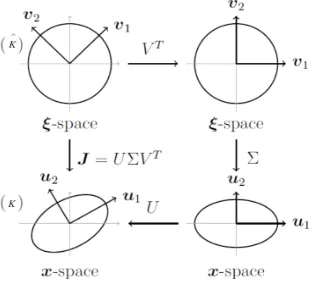
Taking the singular value decomposition
J=UΣVT, Σ = diag(σ1, σ2),
it follows that
K={x: (x−x(ξ0))T U Σ−2UT (x−x(ξ0)) = ˆr2}.
[image:4.612.180.338.373.515.2]so that the orientation of K is determined by the left singular vectors U = [e1,e2], and the size and shape by the singular valuesσ1andσ2(see Fig 2.1). We can quantify
Fig. 2.1. The 2D mapping of a set (Kˆ, a circle) inΩc, to a physical mesh element (K,
an ellipse) inΩp, underx(ξ). The local anisotropy of the transformation is evident from the
degree of compression and stretching of the ellipse.
the size, shape and orientation of an element K, in the continuous sense, using the singular values and left singular vectors ofJ, and the eigenvalues and eigenvectors of the associatedmetric tensor
(2.1) M=J−TJ−1.
The eigenvectors of M are e1,e2 and the eigenvalues µ1, µ2, satisfy µi = 1/σi2 for
i= 1,2 , with
M=UΣ−2UT =
e1 e2
" 1
σ2 1
0
0 σ12 2
#
e1T
e2T
Hence, the circumscribed ellipse of a mesh element will have principal axes in the direction of the eigenvectorse1 and e2, with semi-lengths given by the valuesσ1 =
p
1/µ1 andσ2=
p
1/µ2, (although we note that in the discrete case the shape, size,
and orientation of a mesh element are only partially determined by this metric). The anisotropy of the mesh locally is given by the ratio ofσ1 and σ2. Accordingly, one
natural way measure of the skewnessQs in terms ofJ, which provides a measure of
mesh quality, is
(2.2) Qs=
tr(JTJ) 2 det(JTJ)1/2 =
σ21+σ22
2σ1σ2
=1 2
σ1 σ2
+σ2 σ1
.
This measure, and the circumscribed ellipse of a mesh element, are extremely useful for visualising and analysing the degree of anisotropy [32], as we demonstrate later. We note that many other mesh quality measures exist, for example, those that take in to account small angles [37], [30], and more global measures of mesh quality such as the Kwok Chen metric [38].
2.2. Equidistribution and Alignment. One approach to mesh adaptation is to equidistribute ascalar density functionρ(x)>0,over each mesh cell such that
(2.3) ρJ =θ.
where
(2.4) θ=
Z
Ωp
ρ dx/
Z
Ωc
dξ.
Equation (2.3) is the well knownequidistribution principlewhich plays a fundamental role in mesh adaptation, giving direct control over the size, but not the alignment, of the mesh elements. For one-dimensional mesh generation it uniquely specifies the mesh and is widely used [32], with prescribedρoften given by some estimate of the solution error.
For mesh generation in two or more dimensions the equidistribution principle (2.3) alone is insufficient to determine the mesh uniquely and additional constraints are required [46]. Methods that augment the equidistribution principle with further local constraints are in [2], [1], [28], [29], [36], and other principles for anisotropic mesh adaptation in [47], [10], [17]. A common approach to locally controlled anisotropic mesh generation is to define the desired level of anisotropy through a metric tensorM directly. ThenMis prescribed and the JacobianJof the map is calculateddirectly by enforcing the condition
(2.5) Qa ≡
tr(JTMJ)
2 det(JTMJ)1/2 = 1.
This extends the skewness measure (2.2) and is referred to as thealignment condition
[32]. As it requires that all elements are equilateral with respect to the metric M it allows for direct control of the shape and orientation of a mesh element through an appropriate choice of M. It follows from (2.1) that for any scaled metric tensor M=θM, thatpdet(M)J =θ,for allx∈Ωp, which by (2.3) is equidistribution of
ascalar density function
Huang [28] shows that combining the equidistribution and alignment conditions (2.3)-(2.5) gives
(2.7) J−TJ−1=θ−1M, or equivalently JTMJ=θI.
That is, when the coordinate transformation satisfies relation (2.7), the element size, shape, and orientation are completely determined byMthroughout the domain. The resulting mesh will be aligned to the metric M and equidistributed with respect to the measure ρ, and is referred to as M-uniform [32]. In general there is no unique solution to (2.7) for an apriori givenM, and so in practice this condition can only be enforced approximately. The choice of an appropriate metric tensor is important to the success of this method, and typically those which lead to low interpolation errors are chosen. The simplest choice is to take a scalar matrix monitor function of the form
(2.8) M=ρI.
Using a variational approach this is equivalent to Winslow’s variable diffusion method [55]. In this case, the singular values of M, and hence the semi-lengths of the cir-cumscribed ellipse of a mesh element are equal (i.e., it is a circle) if (2.8) is exactly satisfied and the corresponding mesh is isotropic. In contrast, Huang [29] has derived the exact forms ofMfor which the resulting mesh minimizes the interpolation error of some underlying functionu. Piecewise constant interpolation error can be minimised in the L2-norm if
(2.9) M=κh,1[I+α2h,1∇u∇u T]
where αh,1, κh,1 are explicitly given parameters. For piecewise linear interpolation,
the optimal metric tensor is given by
(2.10) M=κh,2[I+αh,2H(u)],
for suitable parametersκh,2, andαh,2, whereH(u) is the Hessian matrix ofu.
Whilst effective in generating (essentially optimal) anisotropic meshes, these methods require finding the full Jacobian of the map at each step, which necessitates incorpo-rating extra convexity conditions to ensure uniqueness, making the resulting (typically variational) methods challenging to implement. While a scalar matrix monitor func-tion is simpler it can be too restrictive to produce a mesh that is aligned to a physical solution [32]. This begs the question of whether a method that equidistributes a scalar mesh density function is generally capable of producing anisotropic meshes. We demonstrate in the next section that by combining equidistribution of a scalar density function (2.6) with aglobalconstraint, namelyoptimal transport, we can pro-duce suitable anisotropic meshes which are relatively easy to compute. Furthermore, for certain features, we are able to derive analytically the precise form of the metric Mto which these meshes align and show it has a similar form to those metrics given in (2.9) and (2.10) which minimise interpolation error.
Definition 2.1. An optimally equidistributed mappingx(ξ) is one which
mini-mizes the functionalI2, where
I2=
Z
Ωc
|x(ξ)−ξ|2dx,
over all invertiblex(ξ)for which the equidistribution condition (2.3) also holds.
The following result gives both the existence and uniqueness of such a map and a means to calculate it.
Theorem 2.2. (Brenier [4], Caffarelli [11]) There exists a unique optimal
map-ping x(ξ)satisfying the equidistribution condition (2.3). This map has the same reg-ularity asρ. Furthermore, the map x(ξ)can be written as the gradient (with respect toξ) of a unique (up to constants) convex mesh potentialP(ξ, t), so that
x(ξ) =∇ξP(ξ), ∆ξP(ξ)>0.
It is immediate that ifx=∇ξP then the Jacobian matrixJissymmetricand is the
Hessian matrix ofP, i.e. in two-dimensons
J=JT =
xξ xη
yξ yη
=
Pξξ Pξη
Pηξ Pηη
=:H(P).
Furthermore, the Jacobian determinantJ is the Hessian determinant ofP such that in two-dimensional problems
J =xξyη−xηyξ =PξξPηη−Pξη2 :=H(P).
The equidistribution condition (2.3) thus becomes
(2.11) ρ(∇P)H(P) =θ,
which is theMonge-Amp`ere equation(MA). This fully nonlinear equation is generally augmented with Neumann or periodic boundary conditions, where the boundary of Ωc is mapped to the boundary of Ωp [9], [17]. However solutions have also been
attained for non-standard boundary conditions [24] and so it has the potential to be applied to more complex geometries. The gradient of P thereby gives the unique map x. Methods to solve (2.11) are described in [10],[17], [?], and form the basis of effective and robust mesh redistribution algorithms in two and three dimensions [5]. These methods have several advantages in practical applications. In particular, they only involve solving scalar equations, they deal naturally with complex boundaries, and they can be easily coupled to existing software both for solving certain PDEs [9], [6] (see also Section 5) and also for approximating functions in operational data assimilation codes [45].
While these meshes satisfy the local scaling condition (2.3), regions whereρis large will result in small mesh elements and vice versa. However, it is not immediately clear what shape and orientation the elements inherit from (2.11), although in [17] it is shown these meshes minimise the global distortion as measured by the integral of
We study this further here by seeking exact solutions of (2.11) and the corresponding meshes. To do this we use the following result:
Lemma 2.3. For a given scalar function ρ(x), the solution of (2.11) is unique,
and the corresponding mesh has a unique metric tensorM, for which
ρ=pdet(M).
Proof. Givenρ(x), it follows from Theorem 2.2 that the Monge-Amp´ere equation (2.11) has a unique solutionP. Hence we may uniquely construct the Jacobian matrix J=H(P) and metric tensorM=θJ−1J−T.SinceJp
det(M) =θ=ρJ from (2.11), the result follows.
We can calculate the explicit form ofM as follows: Assume that we are considering problems in Rn. Since Jis symmetric its eigenvalues λ
1, λ2, . . . , λn are equal to its
singular valuesσ1, σ2, . . . , σn and its (unit) eigenvectorse1,e2. . .en are orthogonal.
The Jacobian can therefore be expressed in the form
J=λ1e1eT1 +λ2e2eT2 +. . .+λneneTn
implying ρ = θ/J = θ/λ1λ2. . . λn. It follows from (2.7) that the metric tensor M
for which the mesh is M-uniform has the same (unit) orthogonal eigenvectors ei and
eigenvaluesµi=θ/λ2i and can be expressed in the form
(2.12) M=θ λ−12e1eT1 +λ
−2
2 e2eT2 +. . .+λ− 2 n eneTn
.
Observe that this metric tensor is not generally a scalar multiple of the identity matrix and differs from the Jacobian.
3. Alignment to a linear feature. In this section we consider how well the meshes generated by solving (2.11) represent two-dimensional linear features, looking at the alignment, scaling, skewness and anisotropy of the meshes constructed for both single shocks and for shocks meeting orthogonally. These are prototypes of the more complex forms of shocks and fronts found in applications [50],[6]. Our study will centre on certain exact solutions of (2.11). To obtain these solutions we will consider simple domains with periodic boundary conditions. Whilst clearly not representative of many applications, we can still use the results obtained as a good local description of the mesh close to linear regions of more complex features in a more complex geometry.
3.1. Construction of an exact map. Let the scalar densityρ(x) take the form ρ(x) =ρ1(x·e1)ρ2(x·e2) :=ρ1(x0)ρ2(y0).
(3.1)
where e1 = [a, b]T, e2 = [−b, a]T, a2 +b2 = 1. Furthermore, assume that the periodic function ρ1 is large when x·e1 = c, and the periodic functionρ2 is large
whenx·e2=d, for given constantsc, andd, and that they are close to 1 otherwise. Note that the solution of the equidistribution equation (2.1) would be expected to concentrate mesh points along the lines given by either of the conditionsx·e1=c, orx·e2=d.
Theorem 3.1. If the scalar density ρ(x) has the form given in (3.1) then the
resulting mapping the uniquely derived metric tensorMsatisfies (2.12), and the mesh aligns exactly along the linear features.
Proof. To show this result we consider the case where Ωc= Ωp= (0,1)2 and the
solution to (2.11) is adoubly-periodic map from Ωc→Ωp, such thatξ= [ξ, η]∈Ωc,
x= [x, y]∈Ωp. The value ofθ defined in (2.4) is calculated as below.
Lemma 3.2. If θ1 andθ2 are defined as follows
(3.2) θ1=
Z 1
0
ρ1(s)ds, and θ2=
Z 1
0
ρ2(s)ds.
thenθ=θ1θ2.
Proof. By the definition in (2.4)
θ=
Z
Ωp
ρ(x)dx/
Z
Ωc
dξ=
Z 1
0
Z 1
0
ρ1(x·e1)ρ2(x·e2)dxdy/
Z 1
0
Z 1
0 dξdη.
Introducing coordinatesx0=x·e1and y0=x·e2, sincee1 ande2are orthonormal
it follows immediately thatdx dy=dx0dy0, so from double-periodicity ofρwe have
θ=
Z 1
0
Z 1
0
ρ1(x0)ρ2(y0)dx0dy0 =
Z 1
0
ρ1(x0)dx0
Z 1
0
ρ2(y0)dy0 =θ1θ2.
It follows that the Monge-Amp`ere equation (2.11) can be expressed in the form
H(P)ρ1(x0)ρ2(y0) =θ1θ2.
(3.3)
Fortuitously, this fully nonlinear PDE is separable and has an exact solution, from which we can calculate the mesh, the metric tensor and the skewnessQs.
Lemma 3.3. For appropriate periodic functionsF(t)andG(t)given by the
solu-tion of (3.7), there exists a doubly-periodic, separable solusolu-tion to (3.3) of the form
(3.4) P(ξ, η) =F(ξ·e1) +G(ξ·e2).
Furthermore, this solution is unique up to an arbitrary constant of addition.
Proof. Differentiating (3.4) with respect toξandη gives
x=∇ξP =e1TF0+e2TG0.
(3.5)
Differentiating again with respect toξandη we obtain
Pξξ =a2F00+b2G00, Pξη =abF00−abG00, Pηη=b2F00+a2G00.
Hence
H(P) =
e1 e2
F00 0 0 G00
e1T e2T
and
H(P) = (a2F00+b2G00)(b2F00+a2G00)−(abF00−abG00)2 = (b2+a2)2F00G00=F00G00.
(3.6)
Substituting (3.6) into the Monge-Amp`ere equation (3.3) we obtain
F00(ξ0)G00(η0)ρ1(x0)ρ2(y0) =θ1θ2,
whereξ0 =ξ·e1 andη0=ξ·e2.Now by (3.5) it follows that
x0=x·e1=e1T·e1F0+e2T·e1G0 =F0(ξ0), y0=x·e2=e1T·e2F0+e2T·e2G0 =G0(η0). Thus, there is a solution of (3.3) of the form (3.4) providedF andGsatisfy
(3.7) F00(ξ0)ρ1(F0(ξ0)) =θ1α and G00(η0)ρ2(G0(η0)) =θ2/α,
where α is (at this stage) an arbitrary constant. From the identities x0 = F0 and y0=G0 it follows thatx0(ξ0)ρ1(x0(ξ0)) =θ1αand for a suitable constantc1,R1(x0)≡
Rx0
0 ρ1(s)ds=θ1α ξ
0+c
1.Since the map from Ωcto Ωp is doubly periodic,x0(0) = 0
andx0(1) = 1. Thus,c1= 0 and from the definition ofθ1,α= 1. Hence, we have
(3.8) x0 =x·e1=R−11(θ1ξ0) =R1−1(θ1ξ·e1).
A similar identity follows fory0 with related function R2 and constantc2, giving
(3.9) y0=x·e2=R2−1(θ2η0) =R−21(θ2ξ·e2).
These define the functionsF andG, and the uniqueness (3.4) follows from the unique-ness of solutions of the Monge-Amp`ere equation (3.3) with periodic boundary condi-tions [41].
We now calculate the Jacobian of the mapJand the metric tensorM. Note that x=∇ξP =e1TR−11(θ1ξ0) +e2TR2−1(θ2η0)
and
(3.10) J= θ1
ρ1(F0(ξ0))
e1eT1 + θ2 ρ2(G0(η0))
e2eT2
with eigen/singular values
(3.11) λ1=θ1/ρ1, and λ2=θ2/ρ2.
From (2.7), we infer that the mesh will be aligned to the metric
(3.12) M= θ2ρ
2 1 θ1
e1eT1 + θ1ρ22
θ2
e2eT2,
with eigenvalues
These explicit forms forJandMreveal the alignment properties of the map. Specif-ically, the eigendecomposition of Jin (3.10) shows that the semi-axes of the ellipses described in Section 2 are parallel to e1 and e2 and thus align with the linear
fea-tures. The linear features we are aiming to represent arise whenx·e1 =x0=cand
x·e2=y0 =dso that respectively eitherρ1 is large andρ2 is not, orρ2 is large and ρ1is not. This ends the proof of Theorem 3.1.
We can also study the mesh away from the features.
Corollary 3.4. Away from the linear features the mesh is in general isotropic
and its skewness is given explicitly by
(3.14) Qs=
1 2
θ
1ρ2 θ2ρ1
+θ2ρ1 θ1ρ2
Proof. Substituting the expressions from our explicit solution into (2.2) gives
(3.15) Qs=
1 2
θ
1ρ2 θ2ρ1
+θ2ρ1 θ1ρ2
The value of Qs depends upon the relative size of the density functionsρ1 and ρ2,
both locally and globally.
Along the linear features, where either ρ1 1 and ρ2 = O(1), or ρ2 1 and ρ1 = O(1), the mesh elements will be anisotropic and skew. Away from the linear
feature, whereρ1andρ2 are both of order one, the degree of anisotropy and skewness
is controlled by the relative values of the density functions in the entire domain, θ1
and θ2. As these are averaged quantities the ratio is again in general of order one.
We give precise estimates presently for these in two examples below.
3.2. Examples. We now consider two specific analytical examples which illus-trate the theory described above.
3.2.1. Example 1: A single periodic shock. As a first example we consider a periodic array of linear features aligned atπ/4 to the coordinate axes so thate1T =
(1 1)/√2 andeT
2 = (1 −1)/ √
2.As a periodic mesh density we take
(3.16) ρ(x) = 1 +α ∞
X
n=−∞
sech2(α(√2x0−n)) :=ρ1(x0), x0 =x·e1,
with α = 50. This density is concentrated along a set of lines of width 1/50√2 which are parallel to e2, one of which passes through the coordinate origin, and
the others arising when x0 = ±1/√2,±2/√2, . . .. Note that along each such line ρ= 51 +O(exp(−50)) and away from each such line ρ= 1 +O(exp(−50)). A direct calculation gives
θ=
Z
Ωp
ρ(x)dx= 3 +O(exp(−50)),
and
R1(x0) =x0+
1
√
2 ∞
X
n=−∞
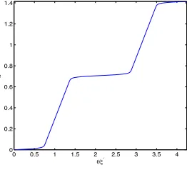
The inverse of R1 can be computed by fitting a spline through the data points
(R1(x0i), x0i), for x0i = √
2i/N0, i = 0, ..., N0. A plot of R−11 is given in Fig. 3.1 for N0 = 1000. Observe that this function is very flat close to x0 = 0,1/√2,√2,
0 0.5 1 1.5 2 2.5 3 3.5 4
0 0.2 0.4 0.6 0.8 1 1.2 1.4
ejv
x
[image:12.612.189.320.153.272.2]v
Fig. 3.1.The functionR−11 for Case 1,θ= 3 +O(exp(−50)).
and mesh points will be concentrated at these values. It follows immediately that θ1=θ, θ2= 1, R2(y0) =y0,and also
ξ0 = (ξ+η)/√2, η0 = (ξ−η)/√2, x= (x0+y0)/√2, andy= (x0−y0)/√2.
Therefore, from (3.8) and (3.9) it follows that
x=√1
2[R −1
1 (θ(ξ+η)/ √
2)−((−ξ+η)/√2)], y= √1
2[R −1
1 (θ(ξ+η)/ √
2)+((−ξ+η)/√2)].
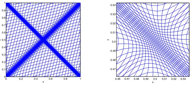
A plot of the resulting mesh is shown in Fig. 3.2(a) with a close-up in Fig. 3.2(b). This mesh is the image of a uniform square computational mesh and has the points (x(ξi, ηj), y(ξi, ηj)), where ξj =ηj =j/(n−1), for i, j = 0, ..., N−1 and N = 60.
We see that not only is the mesh concentrated along the linear features parallel toe2
Fig. 3.2.(Left) A(60×60)mesh generated from the analytical solution of the Monge-Amp`ere
equation for the density function in Case 1. (Right) A zoom of the region along the shock where the density function is large.
[image:12.612.87.420.477.629.2]has a distinctive diamond shape, with each diamond of uniform size and with axes in the directions e1 and e2. The close-up shows the diamonds stretched along the
linear feature and then smoothly evolving into uniform diamonds. The skewness of the mesh can be calculated directly from the Jacobian. The eigenvalues of J(which coincide with the singular values) are given from (3.11) by λ1 = θ/ρ and λ2 = 1.
Ignoring exponentially small terms, we haveλ1= 3/51 within the linear feature, and λ1= 3 away from the linear feature, implying that the skewness measureQsin (2.2)
is given by Qs = 8.529 within the linear feature and Qs = 1.667 outside the linear
feature. Although the specific example given here is not very anisotropic, extremely anisotropic meshes, whilst simple to compute, are difficult to visualise.
Lemma 3.5. A mesh generated by solving (MA) (2.11), with a density function
of the form (3.16), concentrates mesh points along a set of lines of width= 1/α√2, where the mesh is anisotropic with skewness measureQs(3.14) inversely proportional to.
Proof. Ignoring exponentially small terms, the eigenvalues of the Jacobian of the mesh mapping where the density function is at a maximum areλ1 =θ/(1 +α) and λ2= 1, hence the skewnessQs= 1/2((1 +α)/θ+θ/(1 +α)). Sinceα >>1 andθis
order 1
Qs≈
1
√
2θ.
3.2.2. Example 2: Two orthogonal shocks. Consider orthogonal shocks of different widths and magnitudes with the associated scalar densityρ(x) =ρ1(x0)ρ2(y0).
Hereρ1(x0),θ1, andR1(x0) are the same as in Example 1, and
ρ2= 1 + 10
∞
X
m=−∞
sech2(25(√2y0−m)).
A direct calculation givesθ2= 1.8 +O(exp(−25)), and
R2(y0) =y0+ √
2 5
∞
X
m=−∞
[tanh(25(√2y0−m))−tanh(−25m)].
The inverse of R2 can be computed in the same manner as for R1 in the previous
case. Using the same procedures as in Example 1, we have
x=√1
2[R −1
1 (θ1(ξ+η)/ √
2)−R−21(θ2(−ξ+η)/ √
2)],
y=√1
2[R −1
1 (θ1(ξ+η)/ √
2) +R−21(θ2(−ξ+η)/ √
2)].
A plot of the image of a uniform mesh under this map is shown in Fig. 3.3, where we see the excellent alignment of the mesh to the two linear features. Note also the very smooth transition of the mesh from one feature to the other. The eigenvaluesλ1, λ2
(up to exponentially small terms) are:
1. First linear feature alone: λ1= 3/51, λ2= 1.8,
2. Second linear feature alone: λ1= 3, λ2= 1.8/11
0 0.2 0.4 0.6 0.8 1 0
0.1 0.2 0.3 0.4 0.5 0.6 0.7 0.8 0.9 1
x
y
0.46 0.47 0.48 0.49 0.5 0.51 0.52 0.53
0.47 0.48 0.49 0.5 0.51 0.52 0.53 0.54
x
[image:14.612.86.413.103.251.2]y
Fig. 3.3.(Left) A(60×60)mesh generated from the analytical solution of the Monge-Amp`ere
equation for the density function in Case 2. (Right) A zoom of the region along the shock where the density function is large.
4. Outside the two linear features: λ1= 3, λ2= 1.8.
The respective values of the skewness measureQsare
1. Qs= 15.31, 2. Qs= 9.19, 3. Qs= 1.57, 4. Qs= 1.13.
We deduce that away from the linear features and also in the intersection of the two features the mesh in Example 2 is less skew than that of Example 1.
4. Alignment to a radially symmetric feature. In this section we look at radially symmetric features with small length scales. These tend to arise in applica-tions either in the form of singularities (such as in problems with blow-up [13],[9]) or as thin rings, which arise directly as in singular solutions to NLS [43], or approxi-mately as in the curved fronts we study in Section 5. We proceed as in the last section in that we study the alignment and scaling properties of certain exact radially sym-metric solutions of the Monge-Ampere equation. We also study the global geometry and anisotropy of the resulting meshes, including the behaviour close to the domain boundaries. Initially we look at analytic solutions in radially symmetric domains and then see how these solutions perturb in domains without radial symmetry.
4.1. Exact radially symmetric solutions of the Monge-Ampere equa-tion. We begin by considering the form of the Monge Ampere equation (2.11) and mesh mapping in the case of radially symmetric solutions in radially symmetric do-mains. We then consider the nature of the meshes obtained when the density function approximates a Dirac measure. Therefore, we let (x, y) = (Rcos(Φ), Rsin(Φ)) and (ξ, η) = (rcos(φ), rsin(φ)), so thatR =px2+y2, and r = p
ξ2+η2, and assume
that a circle of radius r in Ωc maps to a circle of radius R in Ωp, under the map
R = R(r). Furthermore we assume that the boundary of a disc Ωc maps to the
boundary of a further disc Ωp, such that r = R at the boundary. For a density
function that is locally radially symmetric about the origin
it follows, after some standard manipulations, that there is a radially symmetric solutionP(r) of the Monge-Ampere equation satisfying
Φ =φ, R=Pr and PξξPηη−Pξη2 =
PrPrr
r =
R r
dR dr.
The Monge-Ampere equation (2.11) can be written as
(4.1) ρ(R)R
r dR
dr =θ,
where
(4.2) θ=
R
Ωpρ(R)R dR dΦ
R
Ωcr dr dφ.
We can now study the local structure of the map defined by this expression.
Lemma 4.1. (a) The eigenvectors of the Jacobian of the map are
(4.3) e1=1
r
ξ η
, e2= 1
r −η ξ .
The eigenvectore1is in the direction of increasing rande2 orthogonal to this in the direction of increasing Φ(φ).
(b) The corresponding eigenvalues are
(4.4) λ1= (rψ)0 = dR
dr, and λ2=ψ= R
r =θ/(ρ(R)λ1).
(c) The skewness measure (2.2) takes the form
(4.5) Qs=
1 2 rR0 R + R rR0 .
Proof. Lettingψ:=R(r)/r, it follows from straightforward manipulations, that the Jacobian matrix (expressed in (ξ, η) coordinates) is
J=
"
ψ+ξ2rψ0 ξηψr0
ξηψ0
r ψ+
η2ψ0
r # , = ξ r η r −η r ξ r
(rψ)0 0
0 ψ ξ r −η r η r ξ r ,
and soJ =ψ(rψ)0, hence the result follows.
By (2.12) such a mesh will be aligned to the metric tensor
M= ξ r η r −η r ξ r " θ
(R0)2 0
Integrating (4.1) we obtain
(4.7)
Z R
0
ρ(R0)R0 dR0=θr 2
2.
For given ρ(R) > 0 this expression implicitly defines a unique monotone increas-ing function R(r). Once this function is obtained we can explicitly write down the eigenvalues of the Jacobian matrix and thus quantify the skewness of a mesh element.
NOTE: These results can easily be extended to n-dimensional radially symmetric problems. In this case the generalisation of (4.7) is simply
(4.8)
Z R
0
ρ(R0)(R0)n−1dR0=θr
n
n.
We now consider possible forms for the density functionρ(R) which will concentrate the mesh close to certain features. Specifically, consider
(4.9) ρ(R) = 1 +f(R)
where the functionf(R) is an approximation to a Dirac measure with mass
γ 2 ≡
Z ∞
0
f(R)R dR,
which is large close to R = a and small elsewhere. If a = 0 this density function will lead to a mesh concentrated at the origin, which will be appropriate for resolving the locally radially symmetric singular solutions encountered when studying blow-up type problems [10],[13]. If a >0 this will lead to a mesh concentrated in a thin ring of radius a. This will be appropriate for resolving either a problem with a ring type singularity [43] or (as we shall see when we study the Buckley-Leverett equation in Section 5) the resolution of a front in the solution of a PDE which has locally high curvature.
If we substitute the expression (4.9) into (4.7) we can calculate the relation betweenr andR and hence determine the resulting mesh. It is immediately evident that there are three separate regions (two ifa= 0).
1. Aninner regiongiven byRafor whichρ(R)≈1 and hence
(4.10) R≈√θ r
In this region the mesh is uniform and isotropic and has a scaling factor of√θ. The value ofθdepends upon the boundary conditions and we discuss it presently.
2. A singular region in which R ≈ a where the mesh is concentrated close to the singular feature. The precise nature of this depends on the functionf(R).
3. Anouter regiongiven byRa, away from the singular feature and including the boundary. The form of the mesh in this outer region is given below
Theorem 4.2. Let Raand assume thatρ(R)takes the form (4.9). Then
(a) The mesh is given by the expression
(b) In this region the eigenvalues of the map are given by
(4.12) λ1≈ √
θ/p1−γ/(θr2), λ 2=
√
θp1−γ/(θr2).
(c) The skewness measure is given by
(4.13) Qs≈
1 2
1
1−γ/(θr2)+ 1−γ/(θr 2)
.
Proof. Asf(R) is small ifRa, it follows from(4.7) that ifRathen
R2/2 +γ/2≈θr2/2.
The result (4.11) then follows. To obtain (4.12) and (4.13) note thatρ(R)≈1 in this region and apply Lemma 4.1.
NOTE: We can generalise this result to n-dimensions in which case we have R = (rnθ−γ)1/n
, so spherical shells are mapped to spherical shells, but cuboids are dis-torted.
By applying Theorem 4.2 we can deduce the geometrical form of the mesh in this region. We note that whilst the relation (4.11) maps circles to circles, it does not map squares to squares. Indeed the image of a large square centred on the origin will have a leaf-like shape with the sides of the square mapped closer to the origin than the corners. As r and hence R increases, Qs tends to one, and the mesh becomes
asymptotically isotropic with again a uniform scaling factor of √θ. As r decreases, the value of Qs in (4.13) increases and the mesh becomes more anisotropic. To see
this in more detail, assume that the computational mesh τc is composed of uniform
small squares of sideh aligned with the coordinate axes. A small square lying on a line through the origin parallel to the coordinate axes in the regionr > r1 (R > a)
will be mapped in turn to a small rectangle of sides λ1h and λ2h. In contrast, the
squares on lines at an angle ofπ/4 or similar through the origin will be mapped into diamonds with interior diagonals of length√2λ1hand
√
2λ2h. The smallest angleδ
in such a diamond is given byδ= 2 arctan(λ1/λ2).
To examine the role played by the boundaries we consider a map from a circle in a computational domain of radius r∗ to one in a physical domain of radius R∗. This then determines the value ofθand in turn the level of ainisotropy at the boundary.
Lemma 4.3. (a) If the boundary of a disc of radius r∗ is mapped to one of radius
R∗ andα21 then
(4.14) θ= (R2∗+γ)/r2∗, λ2=R∗/r∗, λ1= (R2∗+γ)/(R∗r∗)
(b) The anisotropy Qs,∗ of the mesh at the boundary is given by
(4.15) Qs,∗=
1 2
1 +γ/R2∗+ 1 1 +γ/R2
∗
.
(c) In the particular case of r∗=R∗,λ1=θ,λ2= 1and
(4.16) Qs,∗=
1 2
θ+1 θ
Hence the skewness of the mesh close to the boundary is small provided thatθ is close to unity.
Proof. These results follow immediately from (4.11) and Lemma 4.1.
4.2. Explicitly Calculated Meshes for Radially Symmetric Features. Now consider a representative density function ρ(R) having the properties of the function in section 4.1 which is simple enough to allow explicit calculation of the mesh. In particular we take
(4.17) ρ(R) = 1 +f(R)≡1 +α1sech2(α2(R2−a2)).
The parameterα1= max(f(R)) (assumed large) determines the density of the point
concentration onto the feature. A measure of the width of the feature is 1/α2a
(as-sumed small) ifa >0 and and 1/√α2ifa= 0. It is immediate that
(4.18) γ=αr=α1/α2 if a= 0, and γ= 2αr if a >0.
Using the expression (4.7) it follows that
Z R
0
(1 +α1sech2(α2((R0)2−a2))R0dR0 =θ r2
2,
and integrating and rearranging both sides we obtain
(4.19) R2+αrtanh(α2(R2−a2)) +αrtanh(α2a2) =θr2=:F(R).
We will now analyse the solution for the cases of (i) singular (blow-up) solution cor-responding toa= 0 and (ii) ring solutions corresponding toa >0.
4.2.1. Meshes for Singular Solutions. When computing solutions with radi-ally symmetric singularities arising over small length scales, such as those observed in the calculation of blow-up solutions [9], [13], we seek meshes which are uniform and isotropic both inside and away from the singular region, and which have a smooth transition between these regions. Such meshes are obtained by this method. To see this, note from (4.19) that fora= 0
(4.20) R2+αrtanh(α2R2) =θr2.
The singular region, in which the mesh is concentrated, has radius of the order of R1= 1/
√
α2 . ForRR1 it follows from (4.20) that
(4.21) R≈rpθ/(1 +α1).
We observe that r and R are linearly related and hence, as required, the mesh is uniform and isotropic in this region. The corresponding region in the computational domain is then given byr < r1where
(4.22) √θr1≈
p
(1 +α1)/α2.
AsRincreases beyond 1/√α2 then tanh(α2R2) rapidly tends towards unity, and the
mesh evolves into the outer region form given in Theorem 4.2. Using Lemma 4.1 we can explicitly calculate the eigenvalues of the transformation, and therefore quantify the level of skewness using the measureQs, in the regions close to the singularity and
in the far field. Specifically,
λ2=R/r≈
(θ/(1 +α1))1/2, for RR1, r−1(θr2−αr)1/2, for RR1,
andλ1=θ/(ρ(R)λ2).The skewness measure Qsis then
(4.23) Qs:≈
1 2
(1+α
1)
ρ +
ρ (1+α1)
, forRR1,
1 2
r2θ
(r2θ−αr)+
(r2θ−α
r)
r2θ
, forRR1.
In the singular region ρ(R)≈1 +α1, so λ1 ≈λ2 ≈
p
θ/(1 +α1),Qs ≈1, and the
mesh is isotropic. If RR1 thenQs approaches one asR → ∞. Note the value of
Qs here is that given by (4.13) with γ =αr and a =R1. As R decreases towards R1 the mesh becomes more anisotropic andQs, as determined implicitly from (4.20)
takes a maximum value Qs,max. This maximum value occurs near R ≈ 2/ √
α2 for
which
(4.24) Qs,max≈
1 2
4 +α
1tanh(4)
4−α1(1−tanh(4))
+4−α1(1−tanh(4)) 4 +α1tanh(4)
.
We now consider two examples of meshes forr∗=R∗= 1/2.
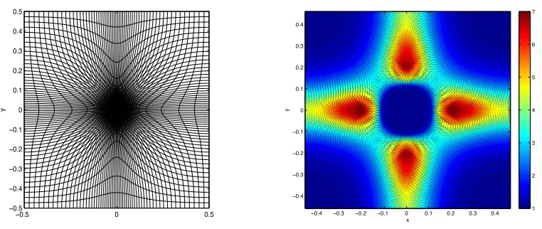
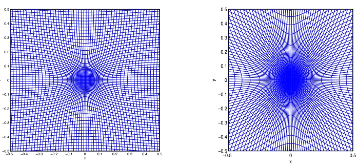
If α1 = 10, andα2= 200 then from (4.14) we have θ= 1.2 and from (4.16)Qs,∗ = 61/60 at the boundary. Hence the mesh has skew elements at the boundary. The elements of maximum skewness are located just outside the blow-up region and from (4.24) Qs,max = 1.9. The resulting mesh as an image of a 60×60 uniform mesh
in the computational domain is plotted on the left in Figure 4.1, and the structure of the intermediate and outer regions is apparent. If α1 = 50, andα2 = 100, then θ = 3 and Qs,∗ = 5/3. At the boundary λ1/λ2 =θ = 3, hence the mesh elements
will be stretched in the radial direction by a factor of 3. In the singular region the elements are isotropic and the elements in the physical domain will be approximately
p
3/51≈1/4 the size of those in the computational domain. The maximum skewness Qs,max= 6.8 and so the mesh elements will be stretched in the radial direction by a
factor of 13. The mesh is shown on the right in Figure 4.1 and shows a much greater degree of skewness. Again we note that much greater skewness would arise than the example presented here for a larger value ofθ. It is interesting to note these meshes
have the same structure as those generated by the Monge-Ampere method to solve PDE’s with blow-up solutions [9].
4.2.2. Ring solution. We now consider the case of a > 0, α1 1, α2 1 so
that ρ ≈1 if |R2−a2| > O(1/a2
2) and ρ ≈1 +α1 otherwise, which leads to mesh
ï0.5 ï0.4 ï0.3 ï0.2 ï0.1 0 0.1 0.2 0.3 0.4 0.5 ï0.5 ï0.4 ï0.3 ï0.2 ï0.1 0 0.1 0.2 0.3 0.4 0.5 x y
ï0.5 0 0.5
[image:20.612.92.440.100.264.2]ï0.5 ï0.4 ï0.3 ï0.2 ï0.1 0 0.1 0.2 0.3 0.4 0.5 x y
Fig. 4.1. The mesh generated from the image of a regular square mesh (60×60) under
the action of a radially symmetric solution of the Monge-Ampere equation fora = 0when
α1 = 10, α2 = 200, θ = 1.2 (left) and when α1 = 50, α2 = 100, θ = 3 showing greater
skewness (right). The leaf like structure of the mesh in the outer region is apparent in both examples.
of√θ.Whena >0 the function (4.19) can be approximated by
R≈ √
r2θ, for rr 1,
q
r2θ−α
r+α1a2
1+α1 , for r1rr2,
√
r2θ−2α
r, for r≥r2,
(4.25)
where the radiir1=
p
θ−1(a2−1/α
2), andr2=
p
θ−1(a2+ 1/α
2+ 2αr) are mapped
toR1=
p
a2−1/α
2andR2=
p
a2+ 1/α
2, respectively. Using (4.4) and (4.25)
λ2≈
θ1/2, for rr
1,
((r2θ−αr+α1a2)/(r2(1 +α1)))1/2, for r1rr2,
((r2θ−2α
r)/r2)1/2, for r≥r2.
(4.26)
λ1≈θ/(ρλ2).
Similarly, the level of anisotropyQs can be approximated by
Qs:=
1 2 1 ρ+ρ
, for r < r1,
1 2
θr2(1+α
1)
ρ(r2θ−αr+α1a2)+
ρ(r2θ−α
r+α1a2)
θr2(1+α1)
, for r1< r < r2,
1 2
θr2 ρ(r2θ−2αr)+
ρ(r2θ−2α
r)
θr2
, for r > r2.
(4.27)
Inside the ring withR a, since ρ≈1,λ1 ≈λ2 ≈ √
θ, soQs≈1 and the mesh is
isotropic. On the ring nearR≈a,ρ≈1 +α1, and the degree of anisotropy depends
on the value α1a2−αr. The larger this value the more anisotropic the mesh. As
a→pαr/(θ−1) thenλ1 →θ/ρ, andλ2→1, hence λ1/λ2 →θ/ρ.Therefore for a
large enough radius of curvatureathe anisotropy approaches that of a linear feature, as expected. As the radius of curvature becomes smaller anda→p
1/α2,ρ→1 +α1,
For example, if a= 0.25 and r∗ =R∗= 1/2, then choosing α1 = 10, andα2= 200,
gives θ ≈ 1.4 and Qs,∗ = 1.05. This results in fairly isotropic elements at the boundary. Inside the ring the mesh elements are isotropic andQs= 1 near the centre
of the ring. Along the ring the elements are anisotropic, andQs = 3.1 at R = 0.25
which is the maximum value. The mesh is shown in Fig. 4.2.
ï0.5 0 0.5
ï0.5 ï0.4 ï0.3 ï0.2 ï0.1 0 0.1 0.2 0.3 0.4 0.5
y
ï0.25 ï0.2 ï0.15 ï0.1 ï0.05 0.05
0.1 0.15 0.2 0.25
[image:21.612.103.492.177.334.2]y
Fig. 4.2. A mesh generated from a radially symmetric solution of the Monge-Ampere
equation when α1 = 10, α2 = 200, θ = 1.4 and a = 0.25(left). An enlargement the ring
feature (right).
If insteadα1= 50, andα2= 100, thenθ≈5 andQs,∗= 2.6 so that at the boundary the mesh elements are skew. Inside the ring the mesh elements are isotropic with a scale factor of √5. However, the maximum value of Qs ≈5.1 does not occur along
the ring, as in the previous example, but just outside the ring where elements are stretched in the radial direction. This can be seen in the mesh plot in Fig. 4.3.
ï0.5 0 0.5
ï0.5
ï0.4
ï0.3
ï0.2
ï0.1 0 0.1 0.2 0.3 0.4 0.5
x
y
ï0.25 ï0.2 ï0.15 ï0.1 ï0.05 0.08
0.1 0.12 0.14 0.16 0.18 0.2 0.22 0.24 0.26 0.28
x
y
Fig. 4.3. A mesh generated from radially symmetric solution of the Monge Ampere
equation when α1 = 50, α2 = 100, θ = 5 anda = 0.25 (left). An enlargement of the ring
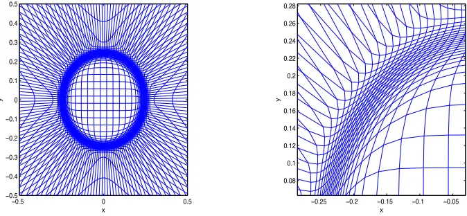
[image:21.612.100.437.478.634.2]4.3. Solutions in domains without radial symmetry. The examples de-scribed in the previous section relate to problems in which we can exactly solve the Monge-Amp`ere equation in a disc, mapping the boundary of a disc to that of another disc. We now consider problems in more general domains. We note that in the outer regionR→√θ r asr→ ∞so that in the limit square domains are mapped to square domains. For most such problems the exact solution of the Monge-Ampere equation is intractable and we must find the solution of this nonlinear elliptic PDE, together with its associated boundary conditions, numerically. This can either be done directly [17], [23], or by using a relaxation method [10], [6]. In this section we will consider, as before, the mesh determined for a radially symmetric feature using the density function (4.17), but now for unit square computational and physical domains centred at the origin. It is shown in [9] that the boundary mapping condition is equivalent to imposing Neumann boundary conditions on the solution to the Monge-Ampere equation. This calculation will allow us to assess the impact of boundary conditions on the alignment of the mesh. In Figure 4.4 (on the left) we see the mesh generated using a numerical solution of the Monge-Ampere equation with Neumann boundary conditions when ΩC = ΩP = S ≡ [−0.5,0.5]2, a = 0.25, α1 = 10, and α2 = 200.
The skewness measure ˆQs for this mesh, which is computed numerically using (2.2),
is shown on the right of Fig. 4.4. A comparison of ˆQs with the skewness measure
ï0.5 0 0.5
ï0.5 ï0.4 ï0.3 ï0.2 ï0.1 0 0.1 0.2 0.3 0.4 0.5
x
y
x
y
ï0.4 ï0.3 ï0.2 ï0.1 0 0.1 0.2 0.3 0.4 ï0.4
ï0.3 ï0.2 ï0.1 0 0.1 0.2 0.3 0.4
[image:22.612.102.471.346.501.2]1 1.5 2 2.5 3
Fig. 4.4. The (60×60) mesh computed numerically for the density function (4.17)
withα1 = 10, α2 = 200, anda= 0.25, with boundaryΩC = ΩP = [−0.5,0.5]2, (left). The
numerically computed skewness measureQˆs (right).
Qsfor the radially symmetric solution in (4.27), reveals that the effects of the square
geometry on the skewness of the mesh are negligible. The skewness is almost radially symmetric for the mesh generated in the unit square, although the skewness of ele-ments that lie along the axisy= 0 and those that lie alongy=xdiffer slightly. The values of Qs at R = 0,R =a, and R = 1/2, are 1, 3.1, and 1.05 respectively. The
values of ˆQsat (0,0), (a,0), (1/2,0), are 1, 3.1, 1.2, where as at (0,0), (a/ √
2, a/√2), (1/2,1/2) they are 1, 3.3, and 1. In Figure 4.5 (on the left) we see the mesh generated numerically when ΩC = ΩP =S, a= 0, α1 = 50,α2 = 100, and (on the right) the
numerically computed skewness measure ˆQs. As in the previous section, this mesh is
ï0.5 0 0.5 ï0.5
ï0.4 ï0.3 ï0.2 ï0.1 0 0.1 0.2 0.3 0.4 0.5
y
x
y
ï0.4 ï0.3 ï0.2 ï0.1 0 0.1 0.2 0.3 0.4
ï0.4
ï0.3
ï0.2
ï0.1 0 0.1 0.2 0.3 0.4
[image:23.612.100.481.101.262.2]1 2 3 4 5 6 7
Fig. 4.5. Numerically computed (60×60) mesh in S for the density function (4.17),
withα1 = 50,α2= 100, and a= 0(left). The numerically computed skewness measureQˆs
(right).
we approach the boundary. Elements that lie along the axisy = 0 and those that lie alongy =xdo not have exactly the same measures of skewness. Recall that for the radially symmetric solution the values ofQsatR= 0, andR= 1/2 are 1 and 5/3, and
the maximum value ofQsis 6.5, and occurs behind the region of blowup. For the
nu-merically computed mesh, along the axisy= 0, the value of ˆQsat (0,0), and (1/2,0),
is 1 and 4.4. Therefore, at the boundary, the skewness is more than double that of the mesh generated from the radially symmetric solution. The maximum skewness
ˆ
Qs= 7.1 is also slightly greater than the radially symmetric case, although we note
that it occurs at the exact same point just behind the region of blow-up. Along the axisy=xthe elements in the numerically computed mesh are not as stretched in the radial direction as in the radially symmetric case. The maximum value of ˆQsis 3 and
occurs just behind the singular region. At the boundary the value is only 1.2. We also obtain similar results for the ring case in the region outside the ring. In particular, whenθexceeds 1 the effects of the geometry become more significant, and the larger the value ofθthe more skew the elements are near the boundary. Ifθis much larger than 1 the elements of greatest skewness occur just outside of the ring and not at the boundary. However, inside the ring and more importantly along the ring the values of
ˆ
Qsand Qs do not differ significantly, hence the geometry of the mesh has very little
impact on the degree of anisotropy in these regions.
curvature, in which case the results of Section 4 can be used to predict the (local) geometry of the mesh.
5.1. Example 1: A prescribed monitor function. Consider the density function
(5.1) ρ= 1 +α1sech2(α2|Ψ|), Ψ =y−0.2 sin(2π(x+ 0.5)).
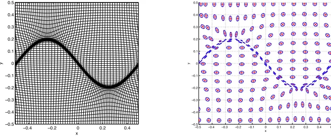
which describes a sinusoidal feature of thin cross-section. We will consider both the lo-cal and the global geometry of the mesh that results when solving the Monge-Ampere equation in a square domain with Neumann boundary conditions in the y-direction and periodic boundary conditions in the x-direction. Such boundary conditions are appropriate for the solution of periodic waves such as (5.1), and arise naturally in many meteorological applications [6]. In Fig. 5.1 the numerically calculated mesh with this density function, for α1 = 20,α2 = 100,θ = 1.2 with the above boundary
conditions, and the corresponding ellipses for the JacobianJ, are shown on the right. It would appear that the eigenvectors ofJare orthogonal and tangential to the curve
ï0.4 ï0.2 0 0.2 0.4
ï0.5 ï0.4 ï0.3 ï0.2 ï0.1 0 0.1 0.2 0.3 0.4 0.5
x
y
ï0.5 ï0.4 ï0.3 ï0.2 ï0.1 0 0.1 0.2 0.3 0.4 0.5
ï0.5
ï0.4
ï0.3
ï0.2
ï0.1 0 0.1 0.2 0.3 0.4 0.5
x
[image:24.612.99.425.312.448.2]y
Fig. 5.1. The numerically computed mesh (60×60) generated for the density function
(5.1) withα1= 20,α2= 100,θ= 1.4, with Neumann boundary conditions n the y-direction
and periodic in the x-direction (left), and the circumscribed ellipses of the JacobianJ(right).
defined as the set for which Ψ(x) = 0. Given that ρ is constant along this curve, it is reasonable to assume there will be no movement of the mesh in that direction, so the eigenvalue corresponding to the tangential eigenvector is estimated to be 1, implying the eigenvalue in the orthogonal direction isθ/ρ. The symmetric matrix˜J corresponds to a metric tensorM˜ with eigenvalues and eigenvectors given by
˜
µ1=ρ2/θ, µ˜2=θ, and ˜e1=∇Ψ/k∇Ψk.
we observe that the eigenvectors are approximately tangential and orthogonal to the shock along the entire curve Ψ(x) = 0. For these regions of maximum curvature of the feature, we instead approximate the eigenvalues of the metric tensor by using the radially symmetric solution of the Monge-Ampere equation studied in Section 4. Specifically we assume that in the region x1 < x < x2, & y < y1, ρ can be well
approximated as part of a radially symmetric feature with density function
ˆ
ρ1= 1 +α1sech2(α2|Ψ1|), Ψ1= ˆR1 2
−a2,
and similarly in the region−x2< x <−x1, &y > y1, by
ˆ
ρ= 1 +α1sech2(α2|Ψ2|), Ψ2= ˆR2 2
−a2,
where ˆR1 =
p
(x+ 0.25)2+ (y+a−0.2)2 and ˆR 2 =
p
(x−0.25)2+ (y−a+ 0.2)2.
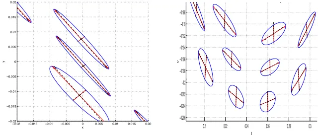
The radius a of the radially symmetric feature is estimated by taking the average radius of curvature along a section of Ψ. We can then approximate the eigenvalues tangential and orthogonal to Ψ as in Section 1.1.4. Note that we calculate θ using the integral of the original density function ρ over the domain, rather than ˆρ. The numerical JacobianJ, when solving PMA using doubly periodic boundary conditions, is compared to an approximation of the Jacobian ˆJ using the eigenvalues from the radially symmetric solution (see Fig. 5.2(left)), for α1 = 20, α2 = 100, θ = 1.4, a = 0.25, and x1 = 0.18, x2 = 0.32, and y1 = 0.18. The circumscribed ellipses for
a number of elements near a region of high curvature are shown together with their semi-axes, which are depicted in red. The semi-axes of the the ellipses associated with ˜
Jare shown in black. If we instead chooseα1= 50,α2= 50, such thatθ= 3, thenJ
ï0.02 ï0.015 ï0.01 ï0.005 0 0.005 0.01 0.015 0.02
ï0.02
ï0.015
ï0.01
ï0.005 0 0.005 0.01 0.015 0.02
x
y
0.2 0.22 0.24 0.26 0.28 0.3
ï0.206 ï0.204 ï0.202 ï0.2 ï0.198 ï0.196 ï0.194 ï0.192 ï0.19 ï0.188
x
[image:25.612.77.397.427.565.2]y
Fig. 5.2. The eigenplot forJ(red) and˜J(black) along the feature, whereΨis approximately
linear (left).The eigenplot forJ(red) andˆJ(black) along the feature in a region of high curvature
(right).
ï0.5 0 0.5
ï0.5
ï0.4
ï0.3
ï0.2
ï0.1
0 0.1 0.2 0.3 0.4 0.5
x
y
ï0.5 ï0.4 ï0.3 ï0.2 ï0.1 0 0.1 0.2 0.3 0.4 0.5
ï0.5 ï0.4 ï0.3 ï0.2 ï0.1 0 0.1 0.2 0.3 0.4 0.5
x
[image:26.612.102.456.107.266.2]y
Fig. 5.3. The computed mesh for the density function (5.1) withα1 = 50, α2 = 50,
θ = 3, anda= 0.25with Neumann boundary conditions in the y-direction and periodic in
the x-direction (left), and an eigenplot ofJ (right).
x
y
ï0.4 ï0.3 ï0.2 ï0.1 0 0.1 0.2 0.3 0.4
ï0.4
ï0.3
ï0.2
ï0.1
0 0.1 0.2 0.3 0.4
1 2 3 4 5 6 7 8 c=1.2
b=1.8
a=3.9
x
y
Q s
ï0.4 ï0.3 ï0.2 ï0.1 0 0.1 0.2 0.3 0.4 0.5
ï0.4 ï0.3 ï0.2 ï0.1 0 0.1 0.2 0.3 0.4
6.2
1.17
9.4 1.08
Fig. 5.4. The value of Qˆs for the numerically computed mesh with density function
(5.1) and Neumann boundary conditions in the y-direction and periodic in the x-direction
whenα1= 20,α2= 100,θ= 1.4, anda= 0.25(left), α1 = 50,α2= 50, θ= 3(right) .
5.2. Example 2: Time Dependant Solution of a nonlinear PDE. We now consider the adaptive numerical solution of the Buckley Leverett equation
(5.2) ut+f(u)x+g(u)y= ˙xux+ ˙yuy+µ4u,
withµ= 1.1×10⁻³. The flux functions are
f(u) = u
2
3(u2+ (1−u)2), g(u) =
1
3f(u)(1−5(1−u)
2),
and the initial data is
u(x, y,0) =
1, (x−0.5)2+ (y−0.5)2< 1 18
[image:26.612.86.423.328.483.2]This model includes gravitational effects in the y-direction. The exact solution is unknown, although numerical results [35], [52], indicate a thin and curved reaction front forms which is our main motivation for studying it here. The solution to (5.2) is computed on the domain [0,1]2 up to time t=0.4. To compute this solution the
mesh is continuously updated by solving a parabolised version (PMA) of the MA equation as described in [10]. The coupled system of the Buckley Leverett equation and PMA is then solved in the computational domain using an alternate procedure with a composite centred finite difference scheme used to discretise both systems. For this calculation we use an arc-length based density function given by
ρ=p1 +|∇u|2.
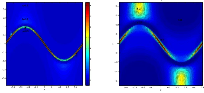
The solution and mesh at t = 0.4 are shown in Fig. 5.5. In Fig. 5.6 a plot of the
0 0.1 0.2 0.3 0.4 0.5 0.6 0.7 0.8 0.9 1
0 0.1 0.2 0.3 0.4 0.5 0.6 0.7 0.8 0.9 1
x
y
x
y
0 0.1 0.2 0.3 0.4 0.5 0.6 0.7 0.8 0.9 1
[image:27.612.83.428.272.422.2]0 0.1 0.2 0.3 0.4 0.5 0.6 0.7 0.8 0.9 1
Fig. 5.5. The numerically computed mesh(80×80)with Neumann boundary conditions
for the Buckley Leverett problem at t=0.4 (left), the solution (right).
circumscribed elipses of the Jacobian for a number of mesh elements reveals that in the region where the density function is large the eigenvectors are tangential and orthogonal to the feature. Furthermore the eigenvectors remain aligned to this feature as the solution and mesh evolves in time. A comparison of the eigenvalues with those associated with a linear feature shows that this is an excellent approximation along regions of the curve that are close to linear (see Fig. 5.7 (left)). Moreover, in regions of high curvature a radially symmetric solution gives a much better approximation. The density function in a region of high curvature is considered to be part of a radially symmetric feature with density function ˜ρ
˜
ρ= 1 +α1sech2(α2|Ψ2|), Ψ2= ˜R2−a2,
where ˜R=p(x−0.62)2+ (y−.72)2,a= 0.2,α
1= 70, andα2= 500. A comparison
of the eigenvalues of the Jacobian with those associated with the density function ˜ρ, which are computed using the radially symmetric solution, are shown in a region of high curvature in Fig. 5.7 (right).
x
y
0 0.1 0.2 0.3 0.4 0.5 0.6 0.7 0.8 0.9 1
0 0.1 0.2 0.3 0.4 0.5 0.6 0.7 0.8 0.9 1
0 0.1 0.2 0.3 0.4 0.5 0.6 0.7 0.8 0.9 1
0 0.1 0.2 0.3 0.4 0.5 0.6 0.7 0.8 0.9 1
x
[image:28.612.85.425.102.262.2]y
Fig. 5.6. The density functionρatt= 0.44for the Buckley Leverett problem (left), and
circumscribed ellipses of the Jacobian for the corresponding mesh (right).
0.885 0.89 0.895 0.9 0.905 0.91 0.915 0.92 0.925 0.93
0.46 0.465 0.47 0.475 0.48 0.485 0.49 0.495 0.5 0.505
x
y
0.41 0.415 0.42 0.425
0.69 0.695 0.7 0.705 0.71 0.715
x
y
Fig. 5.7. A comparison of the eigenvalues of the Jacobian (red) with those corresponding
to the linear solution (black) in a region of low curvature (left), and those corresponding to the radially symmetric solution in a region of high curvature (right).
[image:28.612.96.422.326.474.2]Acknowledgments. The authors thank Phil Browne (University of Reading), Mike Cullen (UK Met Office), Weizhang Huang (University of Kansas), and J F Williams (Simon Fraser University), for many useful suggestions and encouragement. The research of the second and third author is partially supported by NSERC Grant A8781.
REFERENCES
[1] E.F.D. Azevedo and R.B. Simpson, On optimal triangular meshes for minimizing the
gra-dient error,Numer. Math.,59, (1991), 321–348.
[2] M. J. Baines,Least squares and approximate equidistribution in multidimensions, Numer.
Meth. P. D. E.,15, (1999), 605– 615.
[3] H. Borouchaki, P. L. George, F. Hecht, P. Laug, and E. Saltel, Delaunay mesh
genera-tion governed by metric specificagenera-tions. I. Algorithms, Finite Elem. Anal. Des.,25, (1997),
61–83.
[4] Y. Brenier,Polar factorization and monotone rearrangement of vector- valued functions,,
Communications on Pure and Applied mathematics,44(1991), 375–417.
[5] P.A. Browne, C.J. Budd, C. Piccolo and M. Cullen, Fast three dimensional r-adaptive
mesh redistribution, (2013), submitted,
http://people.bath.ac.uk/mascjb/Papers09/paperdraft.pdf
[6] C.J. Budd, M.J.P. Cullen, E.J. Walsh, Monge Amp`ere based moving mesh methods for
numerical weather prediction, with applications to the Eady problem,Journal of
Compu-tational Physics,236, (2013), 247-270.
[7] C. J. Budd, W. Z. Huang, and R. D. Russell, Moving mesh methods for problems with
blow-up, SIAM J. Sci. Comput.,17,(1996), 305–327.
[8] C. J. Budd, W. Z. Huang, and R. D. Russell,Adaptivity with moving grids, Acta Numerica,
18,(2009), 111–241.
[9] C. J. Budd and J. F. Williams,Parabolic Monge-Amp`ere methods for blow-up problems in
several spatial dimensions, J. of Physics A,39, (2006) 5425–5444.
[10] C. J. Budd and J. F. Williams,Moving mesh generation using the parabolic Monge-Amp`ere
equation, SIAM J. Sci. Comput.,31(2009), 3438–3465
[11] L. Caffarelli,InteriorW2,pestimates for solutions of the Monge-Amp`ere equation, Annals
of Mathematics,131(1990), 135–150.
[12] W. Cao,On the error of linear interpolation and the orientation, aspect ratio, and internal
angles of a triangle,SIAM J. Numer. Anal.,43, (2005), 19–40.
[13] H. D. Ceniceros and T. Y. Hou, An efficient dynamically adaptive mesh for potentially
singular solutions, J. Comput. Phys.,172, (2001), 609–639.
[14] L. Chacon, G. Delzanno, and J. Fin,Robust, multidimensional mesh-motion based on
Mon-geKantorovich equidistribution,Journal of Computational Physics,230.1, (2011), 87–103.
[15] J. F. Cossette, and P. K. Smolarkiewicz, A Monge-Amp`ere enhancement for
semi-Lagrangian methods.Computers & Fluids, (2011),46(1), 180-185.
[16] J. F. Cossette, P. K. Smolarkiewicz, and P. Charbonneau, The Monge-Amp`ere trajectory
correction for semi-Lagrangian schemes.Journal of Computational Physics, (2014).
[17] G. Delzanno, L. Chac´on, J. Finn, Y. Chung and G. Lapenta,An optimal robust
equidis-tribution method for two-dimensional grid adaptationbased on Monge-Kantorovich
opti-mization’, J. Comput. Phys.,227(23), (2008), 9841 – 9864.
[18] A. S. Dvinsky, Adaptive grid generation from harmonic maps on riemannian manifolds,
J.Comput. Phys.,95, (1991), 450–476.
[19] L. Formaggia, S. Micheletti, and S. Perotto, Anisotropic mesh adaptation in computational fluid dynamics: Application to the advection-diffusion-reaction and the Stokes problems,
Appl. Numer. Math.,51(4), (2004), 511533.
[20] L. Formaggia and S. Perotto,New anisotropic a priori error estimates,Numer. Math.,89,
(2001), 641–667.
[21] M. Fortin, M-G. Vallet, J. Dompierre, Y. Bourgault, and W.G. Habashi,Anisotropic
mesh adaptation: Theory, validation and applications, ECCOMAS computational fluid
dynamics conference, (1996), 174–180.
[22] P.J. Frey, and F. Alauzet,Anisotropic mesh adaptation for CFD computations,Computer
methods in applied mechanics and engineering,194(48), (2005), 5068–5082.
[23] Brittany D. Froese. A numerical method for the elliptic Monge-Amp`ere equation with
A1432-A1459.
[24] Jean-David Benamou, Brittany D. Froese, and Adam M. Oberman.Numerical Solution
of the Optimal Transportation Problem using the Monge-Ampere Equation, MATH NA
23rd August 2012
[25] P.L. George, F. Hecht, and M.G. Vallet, Creation of internal points in Voronois type
method. Control and adaptation,Adv. Eng. Software,13(5-6), (1991), 303–312.
[26] W. G. Habashi, J. Dompierre, Y. Bourgault, D. Ait-Ali-Yahia, M. Fortin, and M.
Vallet, Anisotropic mesh adaptation: Towards user-independent, mesh-independent and
solver-independent CFD. I. General principles.Internat. J. Numer. Methods Fluids,
32, (2000), 725–744.
[27] F. Hecht,BAMG: bidimensional anisotropic mesh generator,Available from
http://www-rocq.inria.fr/gamma/cdrom/www/bamg/eng.htm, INRIA- Rocquencourt, France, (1998).
[28] W. Huang, Practical aspects of formulation and solution of moving mesh partial differential
equations,J. Comput. Phys.,171, (2001), 753–775.
[29] W. Huang,metric tensors for anisotropic mesh generation,J. Comp. Phys.,204(2), (2005),
633–665.
[30] W. Huang,Measuring Mesh Qualities and Application to Variational Mesh Adaptation,SIAM
J. Sci. Comput.,26, (2005), 1643–1666.
[31] W. Huang, L. Kamenski, and J. Lang,A new anisotropic mesh adaptation method based upon
hierarchical a posteriori error estimates, J. Comput. Phys.229, (2010), 2179–2198.
[32] W. Huang and R. D. Russell,Adaptive Moving Mesh Methods, Springer, (2011).
[33] W. Huang, L. Zheng and X. Zhan, Adaptive moving mesh methods for simulating one
di-mensional groundwater problems with sharp moving fronts,International journal for
numerical methods in engineering,54.11, (2002), 1579–1603.
[34] J.M. Hyman, L. Sheng, and L. R. Petzold, An adaptive moving mesh method with static
rezoning for partial differential equations,Computers and Mathematics with
Applica-tions,46.10(2003), 1511–1524.
[35] K. H. Karlsen, K. Brusdal, H. K. Dahle, S. Evje and K.A. Lie, The corrected operator
splitting approach applied to a nonlinear advection-diffusion problem,Comput. Methods
Appl. Mech. Eng.,167(1998), 239.
[36] P. M. Knupp, Jacobian-weighted elliptic grid generation,SIAM J. Sci. Comput.,17, (1996),
1475–1490.
[37] P. M. Knupp, Algebraic mesh quality metrics, SIAM J. Sci. Comput.,23.1, (2001), 193–
218.
[38] W. Kwok and Z. Chen, A Simple and Effective Mesh Quality Metric for Hexahedral and
Wedge Elements, Proc. 9th International Meshing Roundtable, Sandia National
Laboratories, (2000), 325–333.
[39] X. Li and W. Huang, An anisotropic mesh adaptation method for the finite element solution
of heterogeneous anisotropic diffusion problems,J. Comput. Phys. 229, (2010), 8072–
8094.
[40] X. Li, M.S. Shephard, and M.W. Beal, 3D anisotropic mesh adaptation by mesh
modifica-tion,Comput. Methods Appl. Mech. Engrg.,194(48-49), (2005), 4915– 4950.
[41] G. Loeper, and F. Rapetti,Numerical solution of th
![Fig. 4.4.numerically computed skewness measurewith αThe (60 × 60) mesh computed numerically for the density function (4.17)1 = 10, α2 = 200, and a = 0.25, with boundary ΩC = ΩP = [−0.5, 0.5]2, (left)](https://thumb-us.123doks.com/thumbv2/123dok_us/629179.563815/22.612.102.471.346.501/numerically-computed-skewness-measurewith-computed-numerically-function-boundary.webp)