Towards 5G: A reinforcement learning based scheduling solution for data traffic management

Towards 5G: A Reinforcement Learning-based

Scheduling Solution for Data Traffic Management

Ioan-Sorin Coms

a, Sijing Zhang, Mehmet Aydin, Pierre Kuonen, Yao Lu,

Ramona Trestian, and Gheorghit

˘a Ghinea

Abstract—Dominated by delay-sensitive and massive data appli-cations, radio resource management in 5G access networks is expected to satisfy very stringent delay and packet loss requirements. In this context, the packet scheduler plays a central role by allocating user data packets in the frequency domain at each predefined time interval. Standard scheduling rules are known limited in satisfying higher Quality of Service (QoS) demands when facing unpredictable network conditions and dynamic traffic circumstances. This paper proposes an inno-vative scheduling framework able to select different scheduling rules according to instantaneous scheduler states in order to minimize the packet delays and packet drop rates for strict QoS requirements applications. To deal with real-time scheduling, the Reinforcement Learning (RL) principles are used to map the scheduling rules to each state and to learn when to apply each. Additionally, neural networks are used as function approximation to cope with the RL complexity and very large representations of the scheduler state space. Simulation results demonstrate that the proposed framework outperforms the conventional scheduling strategies in terms of delay and packet drop rate requirements. Index Terms—5G, Packet Scheduling, Optimization, Radio Re-source Management, Reinforcement Learning, Neural Networks.

I. INTRODUCTION

The envisioned applications in the Fifth Generation (5G) of Mobile Technologies (e.g. traffic safety, control of critical infrastructure and industry processes, 50+ Mbps everywhere [1]) impose more stringent QoS requirements like very low end-to-end latency, ultra high data rates, and consequently, very low packet loss rates [2]. To cope with these challenges, access networks should be able to support advanced waveform technologies, mass-scale antennas and flexible Radio Resource Management (RRM) [3]. Alongside standard RRM functions (i.e. power control, interference management, mobility con-trol, resource allocation, packet scheduling [4]), a flexible RRM involves more dynamic functionalities able to adapt to unpredictable network conditions. Some studies have shown an increased interest of integrating Machine Learning (ML) methodologies to learnthe optimal RRM strategies based on some centralized user-centric (i.e. channel conditions, QoS parameters) and network-centric (traffic routing) data [5].

In the context of RRM, the packet scheduler is responsible for sharing the disposable spectrum of radio resources at each Transmission Time Interval (TTI) between active users

I.-S. Coms,a is with Brunel University London, U.K. (e-mail:

[email protected]). S. Zhang is with University of Bedfordshire, U.K. (e-mail: [email protected]). M. E. Aydin is with University of the West of England, Bristol, U.K. (e-mail: [email protected]). P. Kuonen is with University of Applied Sciences of Western Switzerland, Fribourg (e-mail: [email protected]). Y. Lu is with University of Fri-bourg, Switzerland (e-mail: [email protected]). R. Trestian is with Middlesex University, London, U.K. (e-mail: [email protected]). G. Ghinea is with Brunel University London, U.K. (e-mail: [email protected]).

with heterogeneous applications and QoS requirements [6]. The prioritized set of active users to be served at each TTI depends on the type of scheduling rule that is implemented. Different rules may perform differently in terms of packet delay and Packet Drop Rate (PDR) requirements according to various scheduling conditions. For example, the scheduling strategy in [7] minimizes the drop rates at the cost of system throughput degradation. The scheduling rules proposed in [8] improve the packet delays with no guarantees on the PDR performance. Another rule in [9] minimizes packet drops at the expense of higher packet delays when compared with other scheduling strategies. However, most of the proposed rules provide unsatisfactory performance when both delay and PDR objectives are considered concomitantly.

Being motivated by this fundamental drawback of conven-tional scheduling strategies and considering the requirements of 5G networks that need to cater for applications with strict QoS constraints, we propose a flexible RRM packet scheduler able to adapt based on dynamic scheduling conditions. Instead of using a single scheduling rule across the entire transmission, the proposed framework combines multiple scheduling rules TTI-by-TTI in order to improve the satisfaction of stringent QoS requirements in terms of both packet delay and PDR objectives. To make this solution tractable in real time sche-duling, our approach must decide the strategy to be applied at each TTI based on momentary conditions, such as: dynamic traffic load, QoS parameters, and application requirements.

is used to update these functions TTI-by-TTI until learning criteria are fulfilled. Parameterized functions are used to rank the scheduling rule to be applied in each instantaneous state. The scheduler state space needs to be pre-processed in order to reduce the complexity of the proposed RL framework.

A. Paper Contributions

The 5G networks bring the promise of very high data rates and extremely low latencies to enable the support for advanced applications with stringent QoS requirements. However, this is not possible to achieve through the classical methods of RRM, and the integration of ML is seen as a promising solution. In this context, we propose a RL-based optimization mechanism for RRM to enable efficient resource allocation and strict QoS provisioning, bringing us a step closer to 5G. The approach makes use of dynamic scheduling rule selection at each TTI for OFDMA-based downlink access systems. The choice of OFDMA is due to its simplicity and efficiency as well as its wide deployment placing it among the candidate multiple access schemes to be considered in 5G networks [13].

The contributions of this paper are divided in four parts: 1) Flexible RRM Packet Scheduler: We propose a dynamic RRM scheduler able to select, at each TTI, appropriate sche-duling rules according to the momentary network conditions and QoS requirements. The obtained results show significant gains in terms of both delay and PDR satisfaction.

2) RL-based Framework: Here, a RL algorithm is used to learn non-linear functions that approximate the scheduling rule decision at each TTI based on the instantaneous scheduler state. To evaluate the performance of different RL algorithms, five RL algorithms were selected and implemented. Their performance was tested in terms of variable window size, traffic type, objective and dynamic network conditions. 3) Neural Networks (NNs) based Rule Selection:NNs are non-linear functions that take as input the instantaneous scheduler state and output the preference values of selecting each sche-duling rule on that state. Neural networks are used to deal with the continuous and multidimensional scheduler state space. 4) Scheduler State Space Compression Technique:This techni-que aims to reduce the scheduler state space and speed-up the learning procedure when refining the NNs0 weights. In this paper, the focus of the compression procedure is on packet delay and PDR as Key Performance Indicators (KPIs).

The objective of the proposed RL framework is to improve the satisfaction of heterogeneous delay and PDR requirements when scheduling Constant Bit Rate (CBR) and Variable Bit Rate (VBR) traffic types. The CBR and VBR traffic cha-racteristics were chosen in such a way as to cover a wide range of applications (e.g., video, VoIP, FTP, web browsing) and create a more realistic environment with dynamic channel conditions and traffic loads. By building this dynamic and realistic environment, we can evaluate the stability of the learned policies with different RL algorithms.

B. Paper Organization

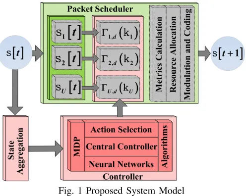
The remainder of this paper is organized as follows: Section II introduces the system model. Section III highlights the preliminaries for the RL framework. Section IV details the im-plemented RL algorithms and the NN function representation.

Fig. 1 Proposed System Model

The performance of the obtained RL framework is evaluated in Section V, and Section VI presents the related work. Finally, Section VII concludes the paper.

II. SYSTEMMODEL

In the proposed system model presented in Fig. 1, an inte-lligent controller decides the rule to be applied by the packet scheduler at each TTI. We consider an OFDMA downlink transmission, where the available bandwidth is divided in Resource Blocks (RBs). Let us consider the set of RBs for a given bandwidth as B={1,2, ..., B}, whereB is the total number of RBs. Additionally, we consider an User Equipment (UE) being characterized by VBR and CBR traffic types with heterogeneous delay and PDR requirements. Also, at each predefined number of TTIs, an UE is able to change its status (idle/active), data rates and QoS requirements. Let us decide that Ut = {1,2, ..., Ut} is the set of active users at TTI t, whereUtis the number of active users.

The packet scheduler (Fig. 1) aims to allocate a set of RBs b ∈ B to user u ∈ Ut in such a way that delay and PDR satisfaction is maximized. We consider the set of objectives O={o1, o2} to be satisfied at each TTIt, where

o1 =DELAY ando2 = P DR. For each user u ∈ Ut, we define the on-line KPIko,u[t]corresponding to objectiveo∈ O and its corresponding requirement as¯ko,u[t]. For useru∈ Ut the objectiveo∈ Ois satisfied at TTItif and only if the KPI

ko,u[t]respects its requirement ¯ko,u[t]. Both, delay and PDR objectives are satisfied when ku[t] = [ko1,u, ko2,u] respects the requirement vector ¯ku[t] = [¯ko1,u,¯ko2,u]. Globally, the proposed solution aims to increase the percentages of TTIs for all active users when the KPI vector k[t] = [k1,k2, ...,kUt]

respects the requirement vector k¯[t] = [¯k1,k¯2, ...,¯kUt], and

consequently, both network objectives are satisfied.

Let us consider the discrete set of scheduling rules asD=

¯

kin a certain measure. The proposed flexible RRM scheduler is able to properly choose the utility functionΓd at each state in order to increase the number of TTIs when ksatisfies k¯.

At the packet scheduler level, B∗Ut ranking values are calculated at each TTI in the metrics calculation block, as in-dicated in Fig. 1. The allocation of RBs involves the selection for each RBb∈ B, the user with the highest priority calculated according to the selected utility functionΓd,u. Then, a proper Modulation and Coding Scheme (MCS) is assigned for the set of allocated RBs of each selected user at each TTI.

A. Problem Formulation

The aim of the proposed solution is to apply at each TTI, the best scheduling ruled∈ Dso that as many as possible KPI parametersk[t]will respect their requirementsk¯[t]. Alongside the simple resource allocation problem, the proposed optimi-zation problem to be solved is more challenging since the rule assignment is required at each TTI, such as:

max x,y

X

d∈D

X

u∈Ut

X

b∈B

xd,u[t]·yu,b[t]·Γd,u(ku[t])·γu,b[t],

s.t.

(1)

X

uyu,b[t]≤1, b= 1, ..., B, (1.a)

X

dxd,u[t] = 1, u= 1, ..., Ut, (1.b)

X

uxd

∗_,u[t] = 1, d∗∈ D, (1.c)

X

uxd

⊗_,u[t] = 0, ∀d⊗ ∈ D\d∗, (1.d)

xd,u[t]∈ {0,1}, ∀d∈ D,∀u∈ Ut, (1.e)

yu,b[t]∈ {0,1}, ∀u∈ Ut,∀b∈ B, (1.f)

where, γu,b[t] is the achievable rate of user u ∈ Ut for RB b ∈ B at TTIt, being calculated as: γu,b[t] =Nu,bbits[t]/0.001 [15], where,Nbits

u,b [t]is the maximum number of bits that could be sent if RB b ∈ B would be allocated to user u ∈ Ut. According to [15], Nbits

u,b [t] is determined as follows: a) at each TTI, the Channel Quality Indicator (CQI) is received for each RB b∈ B and useru∈ Ut; b) a MCS scheme for each RB b ∈ B and UE u ∈ Ut is associated based on CQI; c) using a mapping table N_u,bbits[t] is determined based on MCS. In the maximization problem,xd,u[t]is the scheduling rule assignation variable (i.e. xd,u[t] = 1 when the scheduling rule d ∈ D is assigned to user u ∈ Ut, and xd,u[t] = 0, otherwise). The RB allocation variable is yu,b[t] = 1 when the RB b ∈ B is allocated to user u ∈ B, and yu,b[t] = 0, otherwise. When yu,b[t] = 1, user u ∈ Ut is selected such that u = argmax[Γd,i(ki[t])·γi,b[t]], where i ∈ Ut. The same procedure is repeated for all RBs fromB, until the RBs allocation is finished at TTIt. The constraints in (1.a) indicate that at most one user is allocated to resource RBb∈ B(if the data queue is empty and the scheduling rule does not consider this aspect). One RB cannot be allocated to more than one user, but one user can get more than one allocated RB. Constraints in (1.b) associate for each user a single scheduling rule, and the constraints in (1.c) and (1.d) indicate that the same rule

d∗∈ D is selected for the entire set of active users at TTIt. The solution to the optimization problem in (1) aims to find at each TTI the best scheduling decision xd,u[t] and

resource variable yu,b[t] for all users u∈ Utand RBs b∈ B such that the utilization of resources Bis fully exploited and the satisfaction of objectives O is maximized. Although the PDR objective is correlated with the packet delay, we propose a novel strategy in such a way that: (a) Delay-based Non-congested Case: the delay requirements can be satisfied for most of the active users if proper rules are applied at each TTI; thus, delay minimization represents the primary objective; (b) Delay-based Congested Case:may appear when the KPI vec-torko1[t] ={ko1,1[t], ko1,2[t], ..., ko1,Ut[t]}is not able to reach

the delay requirements anymore and then, we aim to minimize the PDR KPI vector ko2[t] ={ko2,1[t], ko2,2[t], ..., ko2,Ut[t]};

in this case, PDR minimization is the primary objective. The proposed solution is able to detect both cases by considering the multi-objective performance measure or the reward value which is reported at each TTI by the RRM entity.

B. Problem Solution

The constraints in (1.e) and (1.f) make the optimization pro-blem combinatorial. The rule assignment and RBs allocation must be jointly performed in order to keep the linearity of the problem. Moreover, the scheduler has to disseminate which objective to follow according to the delay-based congested and non-congested cases. To solve such a complex aggregate problem, we propose the use of RL framework that is able to interact with the RRM scheduler as indicated in Fig. 1. The RL controller learns to take proper scheduling decisions based on momentary network conditions. This stage is entitled

learning. Then, the exploitation stage evaluates what the controller has learned. Both learning and exploitation stages are managed by a central controller. In order to deal with the optimization problem complexity and large input state, the RL controller engine requires the use of neural networks. In the learning stage, the neural networks are adapted to output better scheduling decisions. The RL algorithms indicate here different ways of updating the NN weights. In Section III, the preliminary elements of RL framework are presented and Section IV elaborates the insights of the RL controller.

III. PRELIMINARIES ONRL FRAMEWORK

The RL framework is used to solve the stochastic and multi-objective optimization problem by learning the approximation of policy of rules that can be applied in real time scheduling to improve the multi-objective satisfaction measure. At TTI

t, the RL controller observes the current state and takes an action. At TTIt+1, a new scheduler state is observed and the reward value is calculated to evaluate the performance of the action performed in the previous state. The reward function together with the scheduler state enhance the decision of the RL controller on the delay-based congestion or non-congestion phases. The previous state, previous action, reward, current state, current action are stored in the Markov Decision Process (MDP) module at the level of RL controller, as shown in Fig. 1. The RL controller explores many state-to-state iterations to optimize the approximation of the best scheduling decisions.

using a single neural network to represent all scheduling rules at once, we propose a distributed architecture of NNs in order to reduce the framework complexity. At each state, the set of NNs providesDoutput values. In the learning stage, the action selection block may choose to improve or to evaluate the NNs outputs according to some probabilities. If the evaluation step is chosen, then the scheduling rule with the highest NN output is selected. Otherwise, the improvement step selects a random rule. The NN weights are updated at each TTI based on the tuple stored in MDP and the type of RL algorithm. During the exploitation, only the evaluation steps are applied.

A. Scheduler State Space

Let us define the finite and measurable set for the scheduler state space as S = SU _{∪ S}C_{, where S}U _{and S}C _{are the} uncontrollable and controllable sub-spaces, respectively. The uncontrollable sub-spaceSU _{cannot be predicted whereasS}C evolves according to the selected rules at every TTI. Let us further define the instantaneous scheduler state at TTI t as a vector: s[t] = [c[t],z[t]], where s[t] ∈ S, c[t] ∈ SC _and

z[t] ∈ SU_{. The uncontrollable elements at TTI t, z ∈ S}U are: CQI reports, number of active users at TTI t, the arrival rates in data queues and the vector of KPI requirements ¯k[t]. The controllable sub-state at TTI t, c ∈ SC _{is denoted by}

c = [k, λ,k,q], where λ[t] = [λ1, λ2, ..., λUt] is the vector

of user data rates being scheduled, k[t] = [k₁,k₂, ...,k_Ut]

comprises the differences between the momentary KPI values

ko,u and their requirements k¯o,u, and q[t] = [q1, q2, ..., qUt]

is the vector of queue lengths. For each user u ∈ Ut, the controllable elements ku[t] = [ko,u−¯ko,u], enable the RL controller to notify when objectives{o1, o2} ∈ Oare satisfied.

B. Action Space

We define the finite action set as A = {a1, a2, ..., aD}, where D is the number of scheduling rules. When the RL controller selects actiona[t] =dat TTIt, the RBs allocation is performed and the system moves into the next state s0 =

s[t+ 1]∈ S according to the following transition function:

c0_(d)=f(s, d), (2)

where c0_(d) = [k0_(d), λ0_(d),k0_(d),q0_(d)] ∈ SC _{is the expected} controllable set at TTIt+1 when applying the scheduling rule

a[t] =d in state s[t]∈ S. The new state s0 ∈ S is obtained based on the uncontrollable elementsz0=z[t+ 1]∈ SU_.

C. Reward Function

As per the original definition [10], the reward represents the expected goodness of applying action a[t] =din states∈ S:

r(s, d)(def=)E

h

Rt+1|s[t] =s, a[t] =d

i

, (3)

whereRt+1 is the reward value calculated at TTI t+ 1. Theorem 1:For any actiona[t] =dapplied in states[t] =s, the reward function will depend on controllable elements from the current and next states, such as: r(s, d) =r(c0_(d),c, d).

Proof 1: The proof is provided in Appendix A. The role of Theorem 1 within the RL framework aims to simplify the reward function calculation and to eliminate the dependency on uncontrollable CQIs. In the absence of Theorem 1, additional pre-processing steps are necessary to

compress the CQI sub-space, which in fact, increases the complexity of the entire RL framework.

The reward function can be further simplified if we consider that, at TTI t+1, the future controllable elements are already known, and consequently, we can say that, c0 =c0_(d). Then, the proposed reward function is calculated as follows:

r(c0,c) =X2

n=1δon·ron(c 0

on,con), (4)

whereδon∈R[0,1]represents the reward weights, whereδo1+

δo2 = 1, con = [kon, λ,kon,q] and kon = [kon,u−k¯on,u].

The weightsδon must stay constant during the entire learning

stage to ensure the convergence of the learned policies [10]. Each sub-reward function in (4) is calculated based on:

ron(c

0

on,con) =

(

1, {r+_on(c0_on), r_o+_n(con)}= 1

r+

on(c

0

on)−r

+

on(con), otherwise.

(5)

The reward expressed above shows the temporal difference in performance for delay and PDR objectives. The proposed sub-reward functions r+

on : R

4·Ut _→

Rare determined according to:r+

on(con) = 1/Ut·

PUt

u=1r −

on(con,u), where the controllable

vector for useru∈ Ut iscon,u= [kon,u, λu, kon,u, qu] and,

r−_on(con,u) =

(

1−kon,u

k_on,u, kon,u≥0,{qu, λu} 6= 0,

1, otherwise. (6)

Basically, when both QoS requirements of all users are satisfied, the reward is 1. Otherwise, the rewards are moderate

(r≥0)or punishments(r <0). We set the delay requirements

¯

ko1 at lower values than initially proposed by 3GPP [16]. In this way, the scheduler is able to provide much lower packet delays than the conventional scheduling approaches.

D. Value and Action-Value Functions

Let us define π: S × A → [0,1] the policy function that maps states to distributions over the action space [17]. In the context of our scheduling problem, we denote the stochastic policy π(d | s) as the probability of action a[t] = d being selected byπin states[t] =s[17], that is defined as follows:

π(d|s) =_P[a[t] =d|s[t] =s]. (7)

Additionally, we define the value function Vπ _{:S →} Rthat measures the value of statesunderlyingπand defined as [17]:

Vπ(s)(def=)_Eπ

h X∞

t=0γ

t

Rt+1|s[0] =s

i

, (8)

where, (1) the process (γt_R

t+1;t ≥ 0) is the accumulated reward value being averaged from state to state by the discount factor γ ∈ [0,1]; (2) s[0] is considered as random such that P(s[0] =s)>0 holds for everys∈ S. The second condition makes the expectation in (8) defined for all states inS. If we also assume that the first action a[0] of the whole process is randomly chosen such thatP(a[0] =d)>0holds for all rules

d∈ Dwhile the following action decisions followπ, then the action-value functionQπ_{:S × A →}

Ris defined as [17]:

Qπ(s, d)(def=)Eπ

h X∞

t=0γ

t_R

t+1|s[0] =s, a[0] =d

i

. (9)

to be redefined and adapted to our scope since the reward in (4) takes as input the consecutive controllable sub-states.

Theorem 2: For any policy π that optimizes (1), we have the new value function Kπ_:SC_{× S}C_→

Rdetermined as:

Kπ(c0,c) =Eπ

h X∞

t=1γ

t−1_R

t|c[1] =c0,c[0] =c

i

, (10)

andJπ _:SC_{× S}C_{× A →}

Ris the new action-value function:

Jπ(c0,c, d) =Eπ

h X∞

t=1γ

t−1_R

t|c[1] =c0,c[0] =c,

a[1] =di, (11)

where the new policy π[d | (c0,c)] states the probability of selecting ruled∈ Dwhen the current state is (c0,c).

Proof 2: The proof can be found in Appendix B. According toTheorem 2, the proposed RL framework learns based on the consecutive controllable states, while eliminating the dependency on other un-controllable elements. This is in fully congruence withTheorem 1 with no need for additional steps to compress the CQI uncontrollable states.

By considering the relations in (8), (10) and (9), (11), respectively, the value and action-value functions can be decomposed according to the temporal difference principle:

Kπ(c0,c) =r(c0,c, d) +γ·Kπ(c00,c0), (12.a)

Jπ(c0,c, d) =r(c0,c, d) +γ·Kπ(c00,c0), (12.b)

wherec00=c[t+2]and the reasonings behind above equations are given in Appendix C.

The optimal value K∗(c0,c) of state (c0,c) ∈ SC _{× S}C is the highest expectable return when the entire scheduling process is started from state (c0,c). Then, function K∗ :

SC _{× S}C _→

R is the optimal value function determined as: K∗(c0,c) = maxπKπ(c0,c) [17]. Similarly, the optimal action-valueJ∗(c0,c, d)of pair(c0,c, d)represents the highest expected return when the scheduling process starts from state

(c0,c)and the first selected action is a[1] =d. Consequently,

J∗(c0,c, d) : SC _{× S}C _{× A →}

R is the optimal action-value function. If we consider that the RL controller acts as optimal at each state, the selection of the best scheduling rule is achieved according to the following equation:

d∗=argmax d0_∈D

[π(d0 |(c0,c)]. (13)

In this case, both value and action-value functions are optimal, and relations (12.a) and (12.b), respectively, become:

K∗(c0,c) =r(c0,c, d) +γ·K∗(c00,c0), (14)

J∗(c0,c, d) =r(c0,c, d) +γ·K∗(c00,c0). (15)

From Appendix B, it can be easily seen that K∗(c00,c0) = maxd0_∈DJ∗(c00,c0, d0). Then, both optimal value and action-value functions can be derived as follows:

K∗(c0,c) =r(c0,c, d) +γ·max d0_∈DJ

∗_(c00_,c0_{, d}0_{), (16)}

J∗(c0,c, d) =r(c0,c, d) +γ·max d0_∈DJ

∗_(c00_,c0_{, d}0_{). (17)}

According to the target values calculated based on (14)-(17) that we would like to achieve at each TTI, the RL framework parameterizes the non-linear functions. Each of these functions

defines the type of RL algorithm. We consider the evaluation of each RL algorithm in order to find the best policy for each parameterization schemes used to compute the on-line PDRs. For our stochastic optimization problem, the optimality of value and action-value functions is not guaranteed. Then, we aim to find the approximations of these functions, such that:

¯

K∗_(c0_,c)≈K∗_(c0_{,c) andJ}¯∗_(c0_{,c, d) ≈J}∗_(c0_{,c, d)for all}

d∈ D. Also, the instantaneous state(c0,c)∈ SC_{× S}C _needs to be pre-processed to reduce the RL framework complexity.

IV. PROPOSEDRL FRAMEWORK A. State Compression

We aim to solve the dimensionality and variability problems of controllable states by eliminating the dependence on the number of active users Ut. This is fundamental for our RL framework, since the input state needs to have a fixed dimen-sion in order to update the same set of non-linear functions.

Theorem 3:At each TTI, the controllable statesc∈ SC_can be modeled as normally distributed variables.

Proof 3:We group the controllable elements as follows:c=

{ko1,ko2, λ,ko1,ko2,q}, where c = {cn}, n = {1, ...,6}. Each component depends on the number of users, such as:

cn={cn,u}, whereu={1,2, ..., Ut}. When nis fixed, each element cn,u can be normalized at each TTItas follows:

ˆ

cn,u=cn,u/(1/Ut·

XUt

u0 cn,u0). (18)

By expanding (18) and fractioning between the pairs, we get the following recurrence relation:

ˆ

cn,u= (cn,u·cn,u+1/ˆcn,u+1). (19)

The normalized setˆcn={cˆn,1,cˆn,2, ...,ˆcn,Ut},∀nis normally

distributed, if and only if, each element cˆn,u is a product of random variables. Equation (19) proves the theorem.

We use the means and standard deviations to represent the distributions of the normalized controllable and semi-controllable elements based on maximum likelihood estima-tors [18]. Let us define the mean function µ(ˆcn) : RUt →

[−1,1] and the standard deviation function σ(ˆcn) : RUt _→

[−1,1]. Based on maximum likelihood estimators [18], these functions are defined as follows:

µ(ˆcn) = 1/Ut·

XUt

u=1ln(ˆcn,u), (20.a)

σ(ˆcn) =

r

1/Ut·

XUt

u=1[ln(ˆcn,u)−µ(ˆcn)] 2

. (20.b)

The same principle for calculating the normalized values and the mean and standard deviations is used for next-state contro-llable elements ˆc0 ={ˆc0_n}. To simplify the controllable state representation, we define the 24-dimensional vector asv∈_Sˆ_,

wherev= [µ(ˆc0_n), σ(ˆc0_n), µ(ˆcn), σ(ˆcn)], andn={1, ..,6}.

B. Approximations of Value and Action-Value Functions

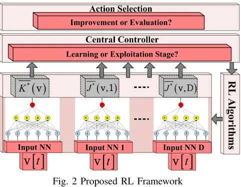
Figure 2 shows the insights of the proposed RL framework. Alongside a number of D neural networks used to approxi-mate the action-value functions, we need an additional neural network to represent the value function. We approximate the optimal action-value functions by defining the function

¯

J∗_{: ˆS × A →}

Fig. 2 Proposed RL Framework

approximator for the optimal value function. Then, the non-linear representations of these functions are defined as follows:

¯

K∗_{(v) =h(θ}

t, ψ(v)), ¯

J∗_{(v, d) =h}d_(θd t, ψ(v)),

(21)

where, {h, h1_{, h}2_{, ..., h}D_{} are the neural networks used to} approximate the value and action-value functions, respectively;

ψ(v)is the feature vector, and{θ, θ1_{, θ}2_{, ..., θ}D_{}is the set of} weights that has to be tuned.

The NN structure is based on two off-line parameterizations: the number of layers and the number of nodes for each layer. Let us defineL the number of NN layers andNl the number of nodes for each layer l ∈ {1,2, ..., L}. If the number of nodes for the input and output layers are known in advance (i.e. N1 = 24, and NL = 1), the number of hidden layers L−2and the number of nodes for each hidden layer must be determined in advance based on a priori testing.

The weights{θ, θ1_{, θ}2_{, ..., θ}D_{} are used to interconnect the} nodes from layer to layer. Let us consider Wl={wb,m, b= 1, ..., Nl, m = 1, ..., Nl+1} the matrix of weights between layers l and l+1. The total number of weights that has to be tuned in the learning stage between layers l and l+1 is

(Nl+ 1)×Nl+1. The compressed controllable states v are passed from layer to layer and they go through a set of non-linear transformations. The output of layer l, becomes [19]:

v(l+1)=ψl+1(WTl ×v

(l)

+), (22)

where,v₊(l)is the biased input state andψl+1is the activation function of layer l+ 1. On the largest scale, the compressed state is propagated through the entire NN according to [19]:

¯

K∗_{(v) =ψ}

L(WTL−1·...·ψl+1(WTl ·...·ψ2(WT1 ·v))). (23)

Similarly, the controllable state v ∈ Sˆ is forwarded through all state-action NNs {h1_{, h}2_{, ..., h}D_{}. The activation function} ψl = (ψl,1, ψl,2, ..., ψl,Nl) is element-wise and the same

function is considered for all nodes. The main idea is to learn

D+1 vectors of weights, but at each TTIt, only two NNs are updated (θt, θdt∗), and a[t] =d∗ is the rule applied in statev. For NN learning purposes, we consider the current state as v0 = [µ(ˆc00n), σ(ˆc00n), µ(ˆcn0), σ(ˆc0n)] ∈ Sˆ and v ∈ Sˆ as a previous state. We aim to update the set of weights {θt, θdt∗}

by reinforcing the error values that are able to evaluate the performance of selecting the output of NN d∗ ∈ D in state

v∈Sˆwhen the current state isv0∈Sˆ. Let us define the value error functione:_R[−1,1]→R[−1,1]and the action-value error function of NNd∈ Dased _:

R[−1,1]→R[−1,1]. These errors are calculated at each TTI based on the following equations:

et(θt−1,v0,v) =KT(v0,v)−K¯∗(v), (24.a)

ed_t(θ_td₋₁,v0,v) =JT(v0,v, d)−_J¯∗_{(v, d), (24.b)}

where, KT _{: ˆS ×S →}ˆ _{Ris the target value function defined}

based on (14) or (16) andJT _{: ˆS ×S × A →}ˆ _{Ris the target}

action-value function calculated according to (15) or (17). Both errors{et,edt}are back-propagated through the neural networks from layer to layer. Let us define the vector of value errorsE(l) _{= [e}(l)

1 ,e (l) 2 , ...,e

(l)

Nl] being back-propagated

to the output of layerl∈ {1,2, ..., L}. These errors are back-propagated based on the following equation [19]:

E(l)=W_lT× 4T_(Ψ0

l+1,E

(l+1)_{), (25)}

where, Ψ0_l+1 = [ψ0_l+1,1, ψ_l0_+1,2, ..., ψ0_l+1,N

l+1] is the deri-vative set and 4[Ψ0

l+1,E

(l+1)_{] = [ψ}0

l+1,1 · e (l+1)

1 , ψ0l+1,2 · e(₂l+1), ..., ψ_l0_+1,N

l+1 ·e (l+1)

Nl+1]. By using (25), the errors are back-propagated from layer to layer and the weights are updated each time based on the gradient descent principle. Then, the weight wt

b,m that interconnects node b = 1, ..., Nl of layerl to node m= 1, ..., Nl+1 of layer l+ 1at TTI t is updated according to the following formula [19]:

w_b,mt =w_b,mt−1+ηt·v

(l)

b ·ψ

0

l+1,m·e

(l+1)

m , (26)

where ηt is the learning rate, v

(l)

b is the state element and ψ0_l+1,m is the derivative function onm∈ {1,2, ..., Nl+1}.

C. RL Algorithms

A set of RL algorithms is used to update the approximations of optimal value and action-value functions. Among all RL algorithms, only five are investigated and used to reinforce the corresponding errors and optimize the NNs{h, h1_{, h}2_{, ..., h}D_} based on dynamic network and traffic conditions.

QV-learning[20] combines the value and action-value func-tions to build its policy by considering a two-step updating process based on (14) and (15), respectively:

KT(v0,v) =r(v, d∗) +γ·K¯∗_(v0_{), (27.a)}

JT(v0,v, d∗) =r(v, d∗) +γ·K¯∗_(v0_{), (27.b)}

where, a[t] = d∗ is the action applied in the previous state

v∈Sˆandr(v, d∗)is the reward function calculated based on (4). The errors are calculated according to (24.a) and (24.b).

QV2-learning[21] keeps the same form of target functions as exposed in (27) with the only difference that, the value function error is back-propagated as follows:

et(θt−1,v0,v) =KT(v0,v)−J¯∗(v, d∗). (28)

QVMAX-learning [21] sets the error calculations and the target function JT_(v0_{,v, d}∗_{) similar to the QV-learning. The} only difference is the target value function, such as:

KT(v0,v) =r(v, d∗) +γ·max d0_∈D ¯

QVMAX2-learning [21] is a combination of QV, QV2 and QVMAX algorithms. The target action-value function

JT_(v0_{,v, d}∗_{) is defined similar to QV-learning as in (27.b),} the target value function KT_(v0_{,v) is determined according} to the QVMAX rule as in (29), the value error et(θt,v0,v) is similar to QV2 and the action-value errored∗

t (θd ∗

t ,v0,v)is determined similar to QV-learning.

For the Actor Critic Learning Automata (ACLA) [22], at each TTI, the value functionK¯∗_{is updated according to (27.a)} and its error is determined based on (24.a). If the value error

et(θt,v0,v)is positive, the actiond∗∈ Din statev∈Sˆwas a good choice and the probability of selecting that action in the future for the same approximated state should be increased. Otherwise, the probability of selecting that action is decreased. The target action-value function is determined as follows:

JT(v0,v, d∗) =

(

1, if e(θt−1,v0,v)≥0, −1, if e(θt−1,v0,v)<0.

(30)

The action selection function from Fig. 2 plays a central role in the learning stage. The trade-off for improvement/evaluation steps is decided by −greedy or Boltzmann distributions. If the−greedy is decided to be used, the actiona[t+ 1]in state

v0 is selected based on the following policy [19]:

π(d|v0) =

(

(_td) ≥t,

hd_(θd

t, ψ(v0)] < t,

(31)

where(_td)is a random variable andtis time-based parameter that decides when the improvement or the evaluation step is applied. If t is very low, then we have more improvements steps. When t gets higher values, the RL controller aims to exploit the output of NNs more. However, the −exploration is not able to differentiate between the potentially good and worthless actions for given momentary states. The Boltzmann exploration takes into account the values of NNs at each TTI, in which, the actions with higher NNs values should have higher probabilities to be selected and the others will be neglected. The potentially good actions for the momentary statev0∈Sˆare detected by using the following formula [19]:

π(d|v0) = exp[h d_(θd

t, ψ(v0))/τ]

PD

d0₌₁exp[hd 0

(θd0

t , ψ(v0))/τ]

, (32)

where τ is the temperature factor that sets how greedy the policy is. For instance, when τ → 0, the exploration is more greedy, and thus, the NNs with the highest outputs are selected. When τ → ∞, the action selection becomes more random, and thus, all actions have nearly the same selection probabilities. Regardless of the type of exploration that is used, the action is selected at each TTI according to (13). Algorithm 1 summarizes the introduced concepts and reasonings.

V. SIMULATIONRESULTS

The proposed framework was implemented in a RRM-Scheduler C/C++ object oriented tool that inherits the LTE-Sim simulator [15]. For the performance evaluation, an infras-tructure of 10 Intel(R) 4-Core(TM) machines with i7-2600 CPU at 3.40GHz, 64 bits, 8GB RAM and 120 GB HDD Western Digital storage was used. The entire framework was simulated using the same network conditions for both learning

Algorithm 1: RRM Scheduler based on RL Algorithms

1: foreach TTIt

2: observestate(c00,c0)∈ SC_{× S}C_{, apply the compression} 3: functions based on (18), (19), (20.a), and (20.b), getv0 ∈_Sˆ_.

4: recallthe previous state and action(v, d),d∈ Dandstore

5: the actual statev0∈Sˆat the controller MDP level 6: calculaterewardr(v, d∗) based on (4), (5) and (6). 7: forwardpropagate states(v0,v) onK¯∗_{(·) =h(θt}

−1, ψ(·))

8: according to (22) and (23)

9: forwardpropagate statev onJ¯∗_{(v, d) =h}d

(θdt−1, ψ(v)),

10: d∈ Dbased on (22) and (23) 11: ifQV algorithm

12: calculatevalue erroret(θt−1,v0,v)- (27.a) and (24.a)

13: calculateerrored t(θtd−1,v

0

,v)- (27.b) and (24.b) 14: ifQV2 algorithm

15: calculatevalue erroret(θt−1,v0,v)- (27.a) and (28)

16: calculateerrored t(θtd−1,v

0

,v)- (27.b) and (24.b) 17: ifQVMAX algorithm

18: calculatevalue erroret(θt−1,v0,v)- (29) and (24.a)

19: calculateerroredt(θtd−1,v 0

,v)- (27.b) and (24.b) 20: ifQVMAX2 algorithm

21: calculatevalue erroret(θt−1,v0,v)- (29) and (28)

22: calculateerroredt(θtd−1,v0,v)- (27.b) and (24.b)

23: ifACLA algorithm

24: calculatevalue erroret(θt−1,v0,v)- (27.a) and (24.a)

25: calculateerroredt(θtd−1,v0,v)- (30) and (24.b)

26: back propagateerroret(θt−1,v0,v)based on (25)

27: updateweightsθt−1 based on (26)

28: back propagateerroredt(θtd−1,v0,v)based on (25)

29: updateweightsθd

t−1 based on (26)

30: // actbased on the learned policy

31: applyd∗=argmaxd0_∈D[π(d0|v0)]based on (31) or (32).

32: end for

and exploitation stages. The obtained results are averaged over 10 simulation runs and the STandard Deviations (STDs) are analyzed in order to prove the veracity of proposed policies. In order to study the impact of the online PDR in the learned policies, different averaging settings are considered.

The aim of the simulations is two-fold: (a) to study the learning performance of five different RL algorithms (QV, QV2, QVMAX, QVMAX2, ACLA) under different traffic types, varying window size, objectives, and dynamic traffic conditions; (b) to study the performance of the proposed RL-based framework and learned policies vs. classical scheduling rules under different objectives, traffic types and network conditions. For the purpose of the performance evaluation, the proposed RL-based framework considers the set of state-of-the-art scheduling rules consisting of EXPonential 1 (EXP1) rule [7], EXPonential 2 (EXP2) and LOGarthmic (LOG) strategies [8] and Earliest Deadline First (EDF) rule [9].

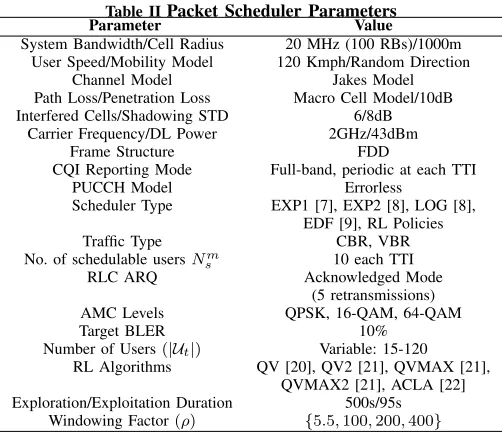
A. Parameter Settings

For the purpose of the simulations, our system model considers the bandwidth of 20 MHz (100 RBs) and the ARQ scheme with maximum 5 retransmissions. Packets failing to be transmitted within this interval are declared lost. Since the packet loss rate is related more to the network conditions, we focus only on the ratio of dropped packets which is related more to scheduler performance. The online PDR KPI

ko2,u[t] for each user u ∈ Ut is calculated as follows:

ko2,u[t] = (

PT

z=tN¯u[z−t])/(P T

Table IIPacket Scheduler Parameters

Parameter Value

System Bandwidth/Cell Radius 20 MHz (100 RBs)/1000m User Speed/Mobility Model 120 Kmph/Random Direction

Channel Model Jakes Model

Path Loss/Penetration Loss Macro Cell Model/10dB Interfered Cells/Shadowing STD 6/8dB

Carrier Frequency/DL Power 2GHz/43dBm

Frame Structure FDD

CQI Reporting Mode Full-band, periodic at each TTI

PUCCH Model Errorless

Scheduler Type EXP1 [7], EXP2 [8], LOG [8], EDF [9], RL Policies

Traffic Type CBR, VBR

No. of schedulable usersNm

s 10 each TTI

RLC ARQ Acknowledged Mode

(5 retransmissions)

AMC Levels QPSK, 16-QAM, 64-QAM

Target BLER 10%

Number of Users(|Ut|) Variable: 15-120 RL Algorithms QV [20], QV2 [21], QVMAX [21],

QVMAX2 [21], ACLA [22] Exploration/Exploitation Duration 500s/95s

Windowing Factor(ρ) {5.5,100,200,400} the number of total transmitted packets andN¯u is the number of dropped packets being caused by higher packet delays than those ones imposed by 3GPP. ParameterT is the time window that is calculated as the ratio between the total number of active users Ut and the maximum number of users Nsm that can be scheduled within one TTI. Then, T = ρ·[Ut/Nsm], where [·] is the integer part and ρ is the windowing factor. The role of ρ is to ensure the PDR satisfaction when Ut is variable. For instance, we have noticed that, when Ut> Nsm, low windowing factors ρ = [5.5,200] provides satisfactory performance for the PDR objective. When Ut <= Nsm, the windowing factor can be increased such as ρ = [200,400]

in order to have larger horizons of time when dropping the packets, while the PDR objective is still satisfied. When ρ > 400, the PDR performance is seriously degraded. However, based on more general traffic settings (Ut is variable during learning and exploitation stages), we would like to find the most convenient range of ρ such that both packet delay and PDR objectives can be maximized. In this sense, we vary the windowing factor inρ={5.5,100,200,400}in order to cover a wider range for both aforementioned cases.

In the learning stage, the packet delay and PDR con-straints are updated at each 1000 TTIs in the range of

¯

ko1,u[t] = {50,100,150,200,250,300}ms and ¯ko2,u[t] = {10−3,10−4,10−5,10−6}, respectively. When the delay ex-ceeds any of these requirements from ¯ko1,u[t], the packets are dropped and declared lost. To obtain better results for the satisfaction of delay, we aim to impose stricter requirements, such that: ¯¯ko1,u[t] = υ · ¯ko1,u[t] and υ = 0.9. Packets exceeding these limits are not discarded, and the proposed policies are able to apply the best rule so that the PDR can be much improved. In order to increase the probability of reaching the terminal states(r(c0,c) = 1)for very high traffic load and low latency requirements, the delay sub-rewards {r+

o1(c 0

o1), r +

o1(co1)} in (5) are modified as follows:

r+_o1(co1) =

(

1, h1/Ut·P Ut

u=1r −

on(con,u)

i

≥κ,

1/Ut·PU_u=1t r−on(con,u), otherwise,

(33)

where, κ∈[0,1]indicates the acceptable limit such that, for

Table III.Controller Parameters

RL Learning Learning Discount Exploration Algs. Rate(ηQ) Rate(ηV) Factor(γ) (, τ)

QV 10−3 ₁₀−5 _{0.99 τ= 10}

QV2 10−3 ₁₀−5 _{0.95 τ= 10}

QVMAX 10−3 ₁₀−5 _{0.99 τ= 10}

QVMAX2 10−3 10−5 0.95 τ= 10

ACLA 10−4 10−4 0.99 = 5·10−5

(1−κ)% of users that are in outage of delay requirements, the delay reward is still maximized. For our simulations, we impose κ= 0.9. When the global reward value is calculated, the same level of importance is given for both delay and PDR objectives, and consequently:δo1=δo2= 0.5.

In both learning and exploitation stages, the number of active users is changed every 1000 TTIs in the domain of

Ut = [15,120] in order to better illustrate the superiority of the proposed policies. The user speed is 30 kmph and the mobility model is considered to be random direction for both learning and exploitation stages. For the interference model, we consider a cluster with 7 cells, and the simulation model runs only on the central cell, with others being used to provide the interference levels. The training stage runs for 500s by using the same user-network-application conditions for all five RL algorithms. The exploitation stages are launched in 10 different simulations of 95s each, and the results are averaged. CBR and VBR traffic types are considered to model a wide range of applications (e.g., video, VoIP, FTP, web browsing) with different traffic characteristics. Thus, the CBR traffic is generated based on the following set of arrival rates λi[t] =

{32,64,128,256,512,1024}randomly generated at each 1000 TTIs (for all active users). The VBR traffic is generated following a Pareto distribution for packet size and geometric distributions for the arrival rates [18]. The obtained policies can provide very high degrees of generalizations, and thus they can be applied to realistic environments. The remaining set of parameters for the RRM packet scheduler is listed in Table II.

B. Optimization of RL Controller

When optimizing the controller, our aim is to find the best parameterization scheme (learning rates, discount factors and exploration parameters) that minimizes the NNs output errors (et,e1t,e2t, ...,eDt ) for a given duration of the learning stage. Different configurations are simulated and Table III illustrates the most suited parameters for each considered RL algorithm. The parameterization of neural networks (L, Nl), l ∈

{1,2, .., L}constitutes another important aspect that has to be considered before launching the learning stage. When the ne-ural network is too flexible (high number of layers and hidden nodes), the complexity is higher, the learning speed slower, and there is a risk to overfit the input state in the sense that, the function approximator will represent not only the interest data, but also the noise in the scheduler state [19]. When the neural network is inflexible (insufficient number of layers and hidden nodes), the system complexity is lower, the RL framework can learn faster, and parts of the scheduler state space may not be represented by the approximator. As a consequence, we get poor generalizations and the function approximator is said to

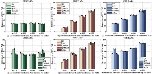
Fig. 3 Learning Performance: Punishment and Moderate Rewards

NN configurations, such as L={3,5,7}, where the number of neurons for each hidden layer was varied in the interval of {50,100,150,200}. Considering under-fitting, over-fitting and system complexity trade-off, and based on preliminary simulations we found out thatL= 3andN2= 100are enough to represent the state space for delay and PDR objectives. For each simulation setting, we considered the same topology of neural networks (i.e. the same numbers of layers, nodes and activation functions). The activation functions for the input and output layers are linear, whilst for hidden nodes, the activation function is tangent hyperbolic [18].

C. Learning Performance

This subsection presents the learning performance of the five considered RL algorithms in terms of the mean percentage of TTIs under punishments and moderate rewards and for varying windowing factor, different objectives (e.g., delay only, PDR only, and both delay and PDR) and different traffic classes (e.g., CBR and VBR). By punishment we understand that the reward is negative at TTIt, such that−1< r <0while in case of moderate reward we have0≤r <1. Thus, for this case, we consider the mean percentage of TTIs under punishments and moderate rewards, such as p(−1< r <0; 0≤r <1). Then,

p1(−1 < ro1 <0; 0 ≤ ro1 < 1) is the mean percentage of TTIs under punishments and moderate rewards for the delay objective; similarly p2(−1 < ro2 < 0; 0 ≤ ro2 < 1) is the mean percentage of TTIs corresponding to PDR objective; and, p₁₂(−1 < r < 0; 0 ≤ r < 1) is the mean percentage of TTIs for both delay and PDR objectives. Figures 3 (a)-(f) illustrate the performance of considered RL algorithms in the exploitation stage when considering the mean percentage of TTIs under moderate rewards and punishments for each traffic class, objective and varying windowing factor.

Figures 3 (a)-(c) show the performance of the RL algorithms in terms of mean percentage of TTIs under punishments and

moderate rewards for varying windowing factor and objectives, for the CBR traffic only. We notice that in the case of delay objective, the percentages p1(−1 < ro1 < 0; 0 ≤ ro1 < 1) remain relatively constant for each of the RL algorithms when varying the windowing factor. However, it can be observed that ACLA performs better than other choices for

ρ={5.5,100}while QVMAX and QVMAX2 perform better forρ={200,400}. When considering the PDR objective only (Fig. 3 (b)), the QV policy accumulates the least amount of punishments and moderate rewards forρ={5.5}and the QV-MAX2 algorithm learns the best when ρ∈ {100,200,400}. However, when both delay and PDR objectives are considered (Fig. 3 (c)), ACLA and QVMAX2 achieve the lowest mean percentage p₁₂(−1 < r < 0; 0 ≤ r < 1) when ρ ∈ {5.5,100,200}and QVMAX2 is the best choice forρ= 400. We observe that the STD ofp₂(−1< ro2 <0; 0≤ro2 <1) becomes higher as ρincreases. This shows that if very large windows are used in the PDR computations, the policies show their limitations in applying appropriate scheduling rules that can maximize the satisfaction of PDR requirements.

The learning performance when scheduling VBR traffic is highlighted in Figs. 3 (d)-(f). QV, QVMAX2 and ACLA perform best for the delay objective (Fig. 3 (d)) forρ= 5.5. Forρ={100,200}, QVMAX, QVMAX2 and ACLA provide a good performance, while QVMAX minimizes p₁(−1 < ro1 < 0; 0 ≤ ro1 < 1) when ρ = 400. The PDR objective (Fig. 3 (e)) satisfaction is achieved for larger periods of time when ρ = 5.5 by the QV policy. However, when increasing the windowing factor,ρ={200,400}, the best candidates are ACLA, QVMAX2 and QV2. When combining both delay and PDR objectives (Fig. 3 (f)), the following policies perform the best: QV, QVMAX2, ACLA for ρ= 5.5, ACLA, QVMAX, QVMAX2 forρ= 100, and QVMAX forρ={200,400}.

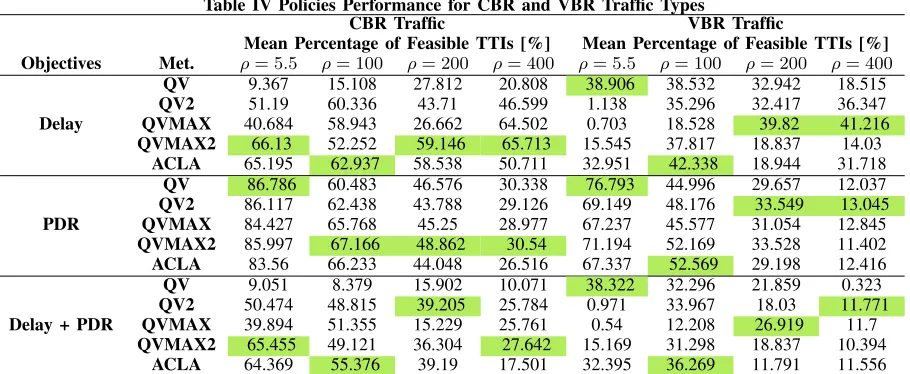
Table IV Policies Performance for CBR and VBR Traffic Types

CBR Traffic VBR Traffic

Mean Percentage of Feasible TTIs [%] Mean Percentage of Feasible TTIs [%] Objectives Met. ρ= 5.5 ρ= 100 ρ= 200 ρ= 400 ρ= 5.5 ρ= 100 ρ= 200 ρ= 400

QV 9.367 15.108 27.812 20.808 38.906 38.532 32.942 18.515

QV2 51.19 60.336 43.71 46.599 1.138 35.296 32.417 36.347

Delay QVMAX 40.684 58.943 26.662 64.502 0.703 18.528 39.82 41.216

QVMAX2 66.13 52.252 59.146 65.713 15.545 37.817 18.837 14.03

ACLA 65.195 62.937 58.538 50.711 32.951 42.338 18.944 31.718

QV 86.786 60.483 46.576 30.338 76.793 44.996 29.657 12.037

QV2 86.117 62.438 43.788 29.126 69.149 48.176 33.549 13.045

PDR QVMAX 84.427 65.768 45.25 28.977 67.237 45.577 31.054 12.845

QVMAX2 85.997 67.166 48.862 30.54 71.194 52.169 33.528 11.402

ACLA 83.56 66.233 44.048 26.516 67.337 52.569 29.198 12.416

QV 9.051 8.379 15.902 10.071 38.322 32.296 21.859 0.323

QV2 50.474 48.815 39.205 25.784 0.971 33.967 18.03 11.771

Delay + PDR QVMAX 39.894 51.355 15.229 25.761 0.54 12.208 26.919 11.7

QVMAX2 65.455 49.121 36.304 27.642 15.169 31.298 18.837 10.394

ACLA 64.369 55.376 39.19 17.501 32.395 36.269 11.791 11.556

learn better under VBR traffic, since the STDs are considerably reduced when compared with the CBR traffic. Moreover, as indicated by (33), we aim to maximize the reward when 90% of active users achieve their delay requirements. In this sense, the RL policy that shows the best performance in terms of learning performance, may not be the best option when we measure the network performance for 100% satisfied users.

D. Policies’Performance

The objective of this subsection is to analyze if the con-sidered RL policies are able to ensure the best performance when measuring the objective satisfaction for all active users. In this sense, we measure the mean percentage of TTIs when 100% of active users satisfy: a) the delay requirements only (p₁(100%)); b) the PDR requirements only (p₂(100%)); and c) both, delay and PDR requirements (p₁₂(100%)).

The results are listed in Table IV for each considered RL algorithm under a varying windowing factor, different objec-tives and traffic classes. The top scheduling policies under each objective and for each windowing factor are highlighted. When the results obtained in Table IV are compared with Fig. 3, a discrepancy between {p₁(100%), p₂(100%), p₁₂(100%)} and 1− {p₁(−1 < ro1 < 0; 0 ≤ro1 <1), p2(−1 < ro2 <

0; 0 ≤ ro2 < 1), p12(−1 < r < 0; 0 ≤ r < 1)} can be observed in the sense that even if some RL approaches are able to provide good performance when minimizing the percentage of TTIs with punishment and moderate rewards, the mean percentage of TTIs when all active users are satisfied is seriously degraded. For example, in Fig. 3(d), for ρ = 5.5, ACLA aims to minimize the number of punishments and implicitly to maximize the number of maximum rewards when 90% of users are satisfied, whereas, in Table IV, QV policy is the best option when measuring p₁(100%). Similarly, in Fig. 3(f), for ρ= 5.5, ACLA and QVMAX2 policies are the best options to minimize the amount of punishment and moderate rewards. However, in Table IV, the QV policy is the one that maximizes p₁₂(100%). Moreover, in Fig. 3(f), QVMAX achieves similar performance as ACLA and QVMAX2 when

ρ = 100. In Table IV, its performance is seriously degraded sincep₁₂(100%) = 12.2, which is three times less than ACLA. These discrepancies are obtained since some policies prefer to select those scheduling rules that aim to keep some users

in outage in terms of packet delay for longer periods. In Table IV, the results show that more than 10% of feasible TTIs for the entire set of RL algorithms and windowing factors are lost when scheduling VBR traffic.

Other discrepancies refer to the performance differences between windowing factors and traffic types. For example, for CBR traffic in the case of the PDR objective when the value of the windowing factor is increased (e.g., 200, 400), QVMAX2 achieves the best performance. Whereas, in the case of VBR traffic, QV2 performs the best under the same settings. Even if the same network and traffic conditions are used when training the NNs under different RL algorithms, the sequence of these conditions differs from one setting of ρ to another. This explains the performance variability of the obtained RL policies under ρ ∈ {5.5,100,200,400} when scheduling CBR and VBR traffic. However, it can be concluded that ACLA is a better option for shorter time windows in PDR computations, whereas the QVMAX and QVMAX2 algorithms can learn better for much longer time windows used in PDR computations.

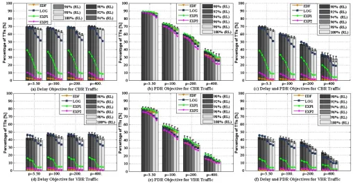
E. Comparison with State-of-the-Art Strategies

The aim of this subsection is to analyze the performance of the proposed RL-based framework and compare it against the conventional scheduling rules, such as EDF, LOG, EXP1, and EXP2. Through this performance evaluation we want to show that by using only one scheduling rule it cannot fully satisfy the objectives under dynamic network conditions and traffic types. Thus, the proposed RL-based framework will select the most suitable scheduling rule to be applied at each TTI based on the current network conditions. The performance of the proposed RL-based framework and the best policies from Table IV are compared against other state-of-the-art scheduling solutions in terms of mean percentage of TTIs when the active users are satisfied in percentage of

q% = {90,92,94,96,98,100} for different objective targets, such as p₁(q), p₂(q), p₁₂(q). The results are collected for CBR and VBR traffic under the three objectives and varying windowing factor and listed in Fig. 4.

Fig. 4 Exploitation Performance: Percentages of TTIs when Delay, PDR, and both Delay and PDR Objectives are Satisfied

CBR (Fig. 4(a)) and VBR traffic (Fig. 4(d)). When scheduling the CBR traffic, more than 10% of feasible TTIs are gained by the proposed framework under all windowing factor settings. Calling the appropriate scheduling rule at each TTI enables all active users to respect the lower delay bound. A degradation of p₁(q) can be observed when scheduling the VBR traffic with ρ = 5.5 for q[%] = {90,92,94}. This is because the main purpose of the obtained policy is to minimize the mean delay for all users with the minimum STD delay values. Some scheduling rules aim to keep some users in outage for longer periods by increasing the STD of packet delays.

The PDR objective for both traffic types under an increasing windowing factorρ,p₂(q)decreases and the results0 variation becomes larger (Figs. 4(b) and 4(e)). However, the proposed framework works best whenq[%] ={90,92,94,96,98,100}. When maximizing the percentages of feasible TTIs when all active users are satisfied in terms of both packet delay and PDR requirements, the proposed framework performs the best as seen in Figs 4(c) and 4(f). By selecting appropriate sche-duling rules for different traffic loads, network conditions and QoS requirements, the proposed framework gains more than

15% of p₁₂(100%) when compared with classical scheduling rules for the CBR traffic type and the windowing factor of

ρ = {5.5,100,200,400}. For the VBR traffic, the proposed framework indicates a gain of about 10%. This is because some packets have larger sizes when compared with CBR.

F. General Remarks

The performance of the RL controller depends on the following factors: the type of RL algorithm, the input data set being used in the training stage, data processing, controller parameterization and the learning termination condition. If the sequence of provided input data is not similar, the performance of the RL algorithms can differ as we observed in Table IV. The training data has to be carefully chosen in order to

permit the controller to explore as many states as possible and to avoid the local minima problems. The input observations must be pre-processed before applying to the RL controller in order to avoid the dependency for some parameters that may change over time, such as the number of active users. The controller setting has to be determined a priori by using extensive simulation results. The NN configuration for our scheduling model makes use ofL= 3layers, where:N1= 24,

N2= 100,N3= 1. Finally, the learning termination condition indicates when the training stage should be stopped. For our simulations, the termination condition is performed after 500s, the moment of time when the errors for all five RL algorithms are nearly the same and the weights of NNs are saved.

VI. RELATEDWORK

One key aspect in obtaining optimal performance within the radio access network is the dynamically scheduling of the limited radio resources. Different radio resource allocation strategies and scheduling rules have been proposed in the literature to optimize the distribution of radio resources among different users by considering the dynamic channel conditions as well as QoS requirements. For example, the EXP1 rule proposed in [7] is able to enhance the PDR at the cost of throughput degradation when scheduling video streaming services. Two rules EXP2 and LOG proposed in [8] are able to minimize the overflow of data queues when compared to Modified Largest Weighted Delay First (MLWDF). However, the MLWDF rule provides poor PDR performance when CBR traffic is scheduled [23]. The EDF strategy in [9] outperforms MLWDF, LOG, EXP1, and EXP2 in terms of PDR with delay degradation when higher real-time traffic load is scheduled.

and packet scheduling [28]–[30]. In many RRM optimization problems, the states (network conditions) and actions (RRM decisions) are continuous and multidimensional variables that increase the complexity of RL algorithms. Different approa-ches are proposed to avoid these drawbacks.

Clustering methods are used in [31] to convert the conti-nuous state space into its discrete representation. In [26], the discrete state space is achieved through fuzzy logic mechanism by using linguistic variables. Another solution is to integrate RL algorithms with artificial Neural Networks, which are able to approximate non-linear functions that map the continuous state into desired scheduling decisions for the proportional-fair rule parameterization [29], [30]. However, some pre-processing tools are needed to compress the NN input state dimension, and consequently, to speed-up the learning process. A form of compression is considered in [28], where the modulation and coding scheme is adapted based on average CQI reports received from all users. This method can be used only in wide-band CQI reporting scenarios, becoming automatically unfeasible when the sub-band reporting is requ-ired. For the self-organizing mechanism proposed in [25], the state compression considers only the conflicting parameters with neighboring cells. Some approaches consider the division of the multidimensional state into smaller sub-states to be approximated as indicated in [32].

VII. CONCLUSIONS

This paper proposes a flexible RRM packet scheduler which is able to adapt based on dynamic scheduling conditions and to enable QoS provisioning. The proposed approach makes use of Reinforcement Learning to determine, for each instantaneous scheduler state, a better scheduling rule to be applied. Additionally, an innovative technique that compresses the controllable momentary state such that the dependency on the number of users is eliminated is also introduced. Through extensive simulation results we have demonstrated that different RL approaches behave differently under varying network conditions and system settings. However, we show that by using the proposed framework together with the best RL policies in the exploitation stage, the proposed RRM scheduler outperforms the classical scheduling rules in terms of both packet delay and PDR objectives.

As part of future work, we plan to investigate the proposed RL framework as a possible solution for the optimization pro-blems that consider non-orthogonal multiple access schemes as well as heterogeneous traffic conditions with strict QoS.

ACKNOWLEDGEMENTS

This work has been performed partially under the fra-mework of the Horizon 2020 project NEWTON (ICT-688503) with funds from the European Union. The authors would like to acknowledge the contributions of their colleagues in the project although the views expressed in this paper are those of the authors and do not represent the project.

APPENDIXA: PROOF OFTHEOREM1

The reward function is decomposed as indicated in (34) when starting with the definition in (3), where, the(∗)property indicates that, the uncontrollable state z[t] = z ∈ SU _can

r(s, d)(3)= E

h

Rt+1|s[t] =s, a[t] =d

i

(2)

= E

h

Rt+1|c[t+ 1] =f(s, d),s[t] =s, a[t] =d

i

=_EhRt+1|c[t+ 1] =c(0d),c[t] =c,z[t] =z, a[t] =d

i

(∗)

= _EhRt+1|c[t+ 1] =c0(d),c[t] =c, a[t] =d

i

=r(c0_(d),c, d). (34)

be reproduced if the controllable elements {c,c0

(d)} ∈ S

C

from the actual and future scheduler states are known. For instance, by having the tuple {λ, λ0_(d)}, the effective SINR can be reproduced, and consequently, the CQI reports for each user can be approximated. The KPI requirements at TTIt k¯

are determined based on the controllable elements {c,c0_(d)}. The arrival bit rates in data queues at TTItare obtained based on the differences between consecutive sizes of queuesq0 and

q. The queue sizes denote here the number of bits from each users, queue being impacted only by the scheduling decision. The arriving bits in data queues depend on the traffic type and are included in the uncontrollable state space. Also, the number of active usersUt at TTIt can be easily determined by simply settingλu= 0for those users in the IDLE state.

APPENDIXB: PROOF OFTHEOREM2

We develop the initial value function as shown in (35). By starting with the definition from (8), the sum of expectations keeps the same value when considering the transition function of controllable elements from (2). The (∗) property has the same meaning as in Equation (34). At TTIt+1 whenc0_(d)=c0, we obtain the value function representation as shown in (10). The action-value function is decomposed as shown below:

Qπ(s, d)(9)=Eπ h X∞

t=0γ

t_R

t+1|s[0] =s, a[0] =d

i

(2)

=_Eπ hX∞

t=0

γtRt+1|c[1] =f(s, d),s[0] =s, a[0] =d

i

=Eπ hX∞

t=0

γtRt+1|c[1] =c0(d),c[0] =c,z[0] =z, a[0] =d

i

(∗)

= _Eπ h X∞

t=0γ

t_R

t+1|c[1] =c0(d),c[0] =c, a[0] =d

i

=Jπ(c0_(d),c, d). (36)

The action-value is developed in (36). At TTIt+1 whenc0_(d)=

c0, the new action-value function is defined as follows:

Jπ(c0,c, d0) =Eπ h X∞

t=1γ

t−1_R

t|c[1] =c0,c[0] =c,

a[1] =d0, a[0] =di (37)

(∗∗)

= Eπ h X∞

t=1γ

t−1_R

t|c[1] =c0,c[0] =c, a[1] =d0

i

,

where,(∗∗)stands with the MDP property.

APPENDIXC: FUNCTIONTRANSITIONS

We want to find a relationship for value and action-value functions in between two consecutive controller states such as