MIAEC: Missing data imputation based on the evidence chain

MIAEC: Missing Data Imputation based on the Evidence Chain

Xiaolong Xu

Data Security & Intelligent Processing

Nanjing University of Posts and Telecommunications

Nanjing, China xuxl@njupt.edu.cn

Weizhi Chong

Information Security, Chinese Academy of Sciences

Beijing, China 1215043122@njupt.edu.cn

Shancang Li, Abdullahi Arabo

Bristol, UK {Shancang.Li, Abdullahi.Arabo}@uwe.ac.uk

Jianyu Xiao*

School of Information Science & Engineering Central South University

Changsha, China Xiaojianyu@mail.csu.edu.cn

Abstract— Missing or incorrect data caused by improper

operations can seriously compromise security investigation. Missing data can not only damage the integrity of the information but also lead to the deviation of the data mining and analysis. Therefore, it is necessary to implement the imputation of missing value in the phase of data preprocessing to reduce the possibility of data missing as a result of human error and operations. The performances of existing imputation approaches of missing value cannot satisfy the analysis requirements due to its low accuracy and poor stability, especially the rapid decreasing imputation accuracy with the increasing rate of missing data. In this paper, we propose a novel missing value imputation algorithm based on the evidence chain (MIAEC), which firstly mines all relevant evidence of missing values in each data tuple, and then combines this relevant evidence to build the evidence chain for further estimation of missing values. To extend MIAEC for large-scale data processing, we apply the Map-Reduce programming model to realize the distribution and parallelization of MIAEC. Experimental results show that the proposed approach can provide higher imputation accuracy compared with the missing data imputation algorithm based on naive Bayes, the Mode imputation algorithm, and the proposed missing data imputation algorithm based on K-nearest neighbor (KNN). MIAEC has higher imputation accuracy, and its imputation accuracy is also assured with the increasing rate of missing value or the position change of missing value. MIAEC is also proved to be suitable for the distributed computing platform and can achieve an ideal speedup ratio.

Keywords: Missing value imputation; data preprocessing; Chain of evidence; Map-Reduce

I. INTRODUCTION

In existing industrial applications, many data mining analysis and processing tools are used to carve potential

useful information for further analysis to improve industry competitive advantage and important findings in scientific research [1, 2]. However, the limitations of data acquisition or improper operation of the data, often lead to data errors, incomplete results, and inconsistencies. Data pre-processing is an indispensable step before data mining. Data preprocessing includes missing data imputation, entity identification, and outlier detection. Missing data padding is an important problem to be solved in data preprocessing. Because of lack of information, the omission of information and man-made operation, some data are missing in the dataset. These incomplete data will affect the quality of data mining and even lead to the establishment of the wrong data mining model, making the data mining results deviate from the actual data.

Pearson R K pointed out that missing data that will lead to three major problems [3]: (1) most of the data processing algorithms at this stage cannot process datasets with missing data. Commonly used algorithms or systems are unable to deal with these incomplete datasets; (2) In the data mining process, in order of performing simple operation to save time, the issue of missing records has often been overlooked, which will lead to poor statistical results;(3) mining datasets with missing records. Many mining methods are very sensitive to the data missing rate of dataset and the reduction of the effective record in the dataset can cause significant decrease or deviation of the mining effect dataset

In industrial applications, more than 80% of the effort is devoted to data preprocessing, so it is necessary to process missing data in order to make full use of the data already collected in machine learning and data mining [4].

common missing value imputation method for MCAR. Since the imputation of NMAR data depends on the prior knowledge of the dataset itself. The effect of different missing types on data classification is discussed in [6].

Due to the difficulty of NMAR data imputation, the current missing value imputation algorithm is for MAR data, relevant attribute values are used to estimate the value of the missing data, However, these methods have their own shortcomings, For example, the linear regression algorithm based on statistical probability and the maximum expectation algorithm must have enough knowledge of the data distribution in the dataset. However, our understanding of most datasets is limited. Based on data mining, such as Bayesian network and k-neighborhood algorithm, the Bayesian network should have a certain knowledge of the domain and knowledge of the data. It is necessary to clear the dependence between various attributes, training Bayesian networks directly with the dataset is quite complex, and KNN algorithm with a high rate of missing cases, the imputation effect will be greatly reduced.

In this paper, by using Map-Reduce programming model a missing data imputation approach based on a chain of evidence (MIAEC) is proposed. MIAEC obtains all relevant evidence of missing data in each tuple of missing data by mining, which is further combined to form a chain of evidence to estimate the missing attribute value. Finally, the value of the missing data is estimated by the chain of evidence. It does not need to master the distribution of data in the dataset, domain knowledge, and does not need to train the dataset estimation model for the imputation to reduce time cost. Most existing algorithms are designed to deal with small datasets on a single machine, but now with the development of information technology, the rapid growth of data, large-scale data processing on a single machine is clearly inappropriate. In MIAEC, Map-Reduce programming model is used to implement the proposed MIAEC algorithm for imputation of large-scale datasets on distributed platforms. Furthuremore, University of California Irvine (UCI) machine learning data is used to carry out the random exclusion of different proportions of the attribute values to get the experimental dataset, and the imputation of the missing data. The results show that MIAEC has high imputation accuracy and imputation stability when imputation values are missing.

II. RELATED WORKS

Zhu et al. [7,8], divide the processing of missing datasets into three main approaches:(1) Delete the missing records. (2) Directly analyze missing datasets, ignoring missing values. (3) Imputation the missing value.

Removal of missing values is to remove the tuples or records from the missing data, using only the complete data tuple or record, so that the analyzed dataset is completed. This approach is simple, especially if the number of missing data is small for the entire dataset, but it is clear that this method will miss some important information due to the deleted

tuples have missing attributes, leaving only the complete tuple, will lead to the analysis of the dataset smaller. D.B. Rubin [5, 9] detailed the risks of deleting tuples of missing data. The further idea is not to delete the missing attribute tuple, nor perform imputation of the missing value, directly in the missing data in the dataset analysis and mining. As described in [10], Bayesian networks are used to process the data. In [11, 12], artificial neural networks are used to process the data, which can reduce the processing-time and avoid the noise caused by the imputation of the missing data. However, the missing data in the dataset may lead to the loss of the useful information, which deviate the mining result. Moreover, [13] concluded that this method is poor in the accuracy of classification when classifying discrete datasets. The work uses the third idea to amputate the missing value.

Most existing missing data imputation methods can be divided into two categories based on the probability of statistical analysis and data mining.

The missing data imputation is to start from the probability of statistical analysis, the probability of missing datasets is analyzed to obtain the missing value of the relevant information, and based on these probability information to fill in the missing data. Linear regression (LR) [14, 15] and Expectation-Maximization (EM) [16] are the most common methods based on probability. For LR and EM parameter methods, if the data distribution of the dataset being processed is not well understood, this will result in an estimate of the deviation. However, in real life, we have a limited understanding of the dataset to be processed. If we compare the data distribution of the dataset, choose the appropriate parameters, and then the missing value of the imputation effect is quite good. But like the EM method even for the dataset of data distribution to understand, the parameter convergence is very slow and time-consuming.

Bayesian classification is also a common algorithm for imputation of missing data [17]. Naive Bayes classification results can be compared with the decision tree algorithm and neural network classifier [18]. The naive Bayesian classification algorithm used for imputation of the missing value is based on the Bayesian theorem formula to estimate the value of missing data [17]. The estimated value of each missing data depends on the value of the other attributes in its tuple. The core formula is as follows:

( | ) ( ) ( | )

( )

P X C P C

i i

P C X

i  _{P X}

(1)

In Equation (1) 1, C

i represents an imputation value of

the missing value estimate, and X represents the value of other attributes in the tuple where the missing value is located. Since P X( ) is a constant for all classes, as long as

( | ) ( )

P X C P C

i i is computed. Naive Bayes has a

conditional independence hypothesis. Therefore, P X C( | )

i

1

( | ) n ( _K| _i)

k

P X C P X C

i 



The algorithm searches the entire dataset for each missing valueP C( |X)

i , taking the maximum probability C

i as imputation value of the missing value. The method is

simple and easy to implement, and the imputation effect is also good. In practical, the relationship between the attributes of datasets is not independent of each other, hence the limitations of using Naive Bayes.

Mode imputation based on statistics is one of the simplest missing data imputation methods. The mode is a measure of central tendency, the mode is the most frequent of values in dataset. It can reflect the basic distribution of data in dataset. So we can choose the most frequent values to imputation the missing data. This method is characterized by simple and easy, however, when there is a complex relationship between the data in the dataset, the method is not good.

Machine learning is the most commonly used method for imputation of missing data in missing dataset. The main aim of using data mining for imputation in missing data is to extract useful information from the original dataset to build the prediction model based on this useful information for further estimating the value of missing value from the predicted model. A number of algorithms based on data mining have been reported, such as k-nearest neighbor (KNN) [19, 20], Bayesian network [21], rough set method [22], etc. There are various algorithms to form a complex combination of algorithms; in [23] the decision tree algorithm and the maximum expectation algorithm are combined to form a new algorithm. This algorithm makes use of the higher classification accuracy of the decision tree, which makes the filling effect very good, with higher classification accuracy; as well as in the original algorithm on the innovative algorithm. In [24], an incomplete data clustering algorithm, MBOI, was proposed, which defines the set of constraint tolerance sets for the incomplete dataset of categorical variables. It can be used to estimate the overall difference of incomplete data objects from the set point of view degree, and further imputation in the missing data based on the result of incomplete data clustering. The algorithm has a good effect on the accuracy of the imputation and the time efficiency of the algorithm.

KNN is based on distance data classification algorithm, which searches the entire dataset to find the k data tuples closest to a given data tuple. KNN is able to mark the tuples with missing data as missing tuples, and then the complete data tuple in the dataset is used as the training dataset, searching for the k data tuples nearest to the missing tuples in the entire training dataset, and finally performing imputation of the missing tuples according to the k data tuples. In practice, KNN has very high classification accuracy, experiments in [20] demonstrated that the K-nearest neighbor algorithm performs well in the absence of DNA

microarray data. However, KNN algorithm has its own shortcomings, when the dataset has a large percentage of missing data, KNN filling accuracy will be greatly reduced.

III. MISSING VALUE IMPUTATION ALGORITHM

A. Related Definitions

Let D denote a dataset with m rows and n columns， which means D has m data tuples. Each data tuple has n

attributes, and the dataset can be defined as

1 2 3

{ , , ,..., _n}

D A A A A (3) in which A_i(1 i n) is the i-th column attribute of the dataset D.

Data tuples in the dataset can be defined as

Dj={V Aj( i) |1 j m,1 i n} (3) where X_{j i}（_, 1 j m,1 i n）represents the value of the

j-th row i-th column attribute of the dataset D. Let the

i-th attribute of the j-th tuple in Dbe V A_j( _i).

Definition 1. The missing model is defined as follows

,(1 ,1 )

( )

'?'(1 ,1 )

j i

j i

X j m i n

V A

j m i n

   



 _{   }



= (5)

in which V A_j( _i)'?' denotes that the i-th attribute value of the j-th tuple is missing.

If a data tuple includes V A_j( _i)'?' , then the data tuple is believed as ‘incomplete data tuple’ and can be described by

Zj{ (V Aj i) |V Aj( i)'?',1 j m,1 i n} (6)

If the array tuple does not include V A_j( _i)'?' , then the array tuple is believed as ‘complete data tuple’, and can be denoted as

Rj { (V Aj i) |V Aj( i)!'?',1 j m,1 i n} (7)

The non-missing data in an incomplete data tuple is the associated attribute value of the missing data in the incomplete data tuple.

Definition 2: Let the set of combinations of the associated attribute values for the missing data as the chain of evidence to estimate the value of the missing value

Sj { ( , ) |1C y u  y n,1 u y} (8)

the y complete attribute values. It is recorded as the evidence of the estimated missing value.

The main goal of the algorithm is to estimate the value of the missing data in the j-th data tuple by the set S_j.

In each data tuple M_i(1 i m) of dataset D, there is a set of attributes, which is assumed to be A.The data tuple

(1 )

i

M  i m contains A, iff AM_i(1 i m),

the rule is formed as AB in the tuple M_i(1 i m)of the dataset D , Among them, AD , BD , A  ,

B , and A  B , All tuples in dataset D contain set

A and set B with the ratio P A( B).

Definition 3: the support count S represents the number of a set in the dataset, and then the support count of the rule

AB in the whole dataset D is defined as:

( ) ( )

S AB P AB (9) Definition 4: Dataset D contains both attribute value set A and contains attribute value set B data tuple ratio

isP B A( | ), the credibility of the rule AB in the whole

dataset D is defined as:

F A( B)P B A( | ) (10) Credibility is calculated as:

( )

( ) ( | )

( )

S A B

F A B P B A

S A



  

(11)

B. MIAEC Algorithm

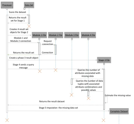
MIAEC is based on the set of associated attribute value combinations of missing data as a chain of evidence to estimate the value of missing data. According to the idea of data mining, there is a certain relationship between data attribute values in large-scale datasets. In the imputation process, the algorithm will first estimate the missing value of the imputation value, the algorithm scans each data tuple in the entire dataset, marking tuples with missing values ‘?’ as incomplete data tuples, and combine the different associated attribute values of the missing data in the incomplete data tuple as evidence of the estimated missing value. So that a large number of combination of the relevant attributes for missing data in the incomplete tuple constitute the estimated missing data value of the chain of evidence. The algorithm scans the entire dataset again and counts the combination of attribute values in all data tuples, and uses the relevant theorem in the prerequisite knowledge to calculate the value of the missing data. The core task of the algorithm is to calculate the reliability of each estimated missing value in the chain of evidence. Thus, gives the sum of the confidence of all the evidence for the estimated missing data, the maximum estimate of the sum of the confidence values is selected as the imputation value.

MIAEC algorithm includes following five stages:

Stage 1. The algorithm first scans the dataset D to uniquely identify I_k(1 k m) for each data tuple D_j, then gives the position M_h(1 h n) of missing data for each

incomplete data tuple to determine which attribute data in the tuple is missing and output the marked dataset. The output data format is (I M D_k, _h, _j).

Stage 2. This stage contains four parallel modules:

Module 1. The algorithm first scans the result file created at Stage 1 to compute the set S_j of combinations the complete data R_j in incomplete data tuple Z_j(1 j m), which will serve as the evidence chain for estimating the missing data values. The result will be used as the chain of evidence to estimate the missing data. The output data format is (I ,M ,S_{k h j}).

Module 2. The module calculates the probability P p( )

of the possible values of the missing values p in each missing tuple from the complete data tuple and the output data ( , ( ))p P p .

( ) ( ) K p

P p m

 (12)

In (12), formula K() represents the count andK p( )

denotes the possible value of the missing value p the number of occurrences of the same missing location in each data tuple, and m denotes the number of data tuples.

Module 3. The module counts the number O_j of the dataset of complete data combination S_j for each data tuple in the entire dataset and will be used in the probability query for the missing data value estimation in the following steps. The output data format is (S O_j, _j).

Module 4. The algorithm counts the number of complete sets of data S_j and missing data in the incomplete data tuple Z_j(1 j m) in the same data tuple, that is T_j.

( ( ) '?'(1 ,1 )

{ ( , ) | 1 ,1 })

j j i j

T K V A j m i n S

C y u y n u y

      

     (13)

The format of the output is （S M_i, _h, ,p T_j）.

Stage 3. at this stage, the evidence chain (I ,M ,S_{k h j}) of estimated missing data created in module 1 at stage 2 will be connected with the possible value ( , ( ))p P p of output

missing data in module 2 at stage 2.The

probability P p( ) that the associated attribute value combination C y u( , ) of missing data in each incomplete data tuple Z_j(1 j m) and each possible padding value p

Stage 4. At this stage, the number O_j of the set S_i of the associated attribute value combinations in the incomplete data Z_j(1 j m) in which the missing data

( ) '?'(1 ,1 )

j i

V A   j m  i n is located in the result file of the Stage 2 module 3 according to e at the Stage 3 result file. According to the results file of Stage 3 S_i and p，and in the results of the Stage 2 module 4 to find the associated attribute value set S_i and missing data possible values p in the entire dataset the number of simultaneous appearances

j

T .According to the above preliminary knowledge, in the incomplete data tuple Z_j(1 j m), we can compute the

probability that all possible missing data values are taken from the setS_iof the associated attribute value combinations.

( )

( ) ( | )

( )

i

i i

i

S p S

F S p P p S

S S



  

（14）

We choose the maximum estimate of the confidence

( _i )

F S p as the final imputation value.

Stage 5. The algorithm imputation the original missing dataset D with the possible values of the missing data estimated at Stage 4.

Figure shows the timing diagram of the algorithm

Processor Data Set

Scans the dataset

Returns the result set for Stage 1

Module 1 File Creates 4 result set

objects for Stage 2

Request connection

Connection

Stage 3 File Module 2 File Module 3 File Module 4 File

Create a phase 3 result object

Stage 4 sends a query message

Queries the number of attributes associated with

missing data

Queries the number of data tuples with associated attribute combinations and

possible values

Returns the result dataset

Estimate the missing value

Complete Dataset Stage 5 Imputation the missing data set

Module 1 and Module 2 connection

Returns the result set

C. Map-Reduce Parallelization of Algorithms

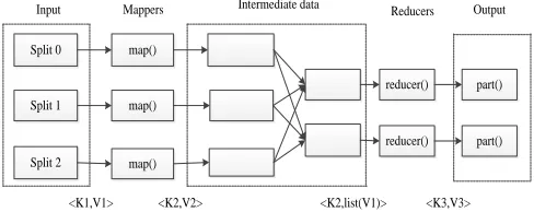
Map-Reduce adopts a divide-and-conquer strategy for large-scale datasets. The core of MapReduce's parallelization is Map and Reduce, the Map-Reduce computing framework divides the dataset into a number of small files with the same size and assigns them to different nodes. Each node performs Map calculation, and the results are sorted and merged. The same Key values are put in the same set Reduce calculation [19]_{. Figure 2 shows the} implementation process of Map-Reduce.

Split 0

Split 1

Split 2 map()

map() map()

reducer()

reducer()

part()

part()

Input Mappers Intermediate data Reducers Output

<K1,V1> <K2,V2> <K2,list(V1)> <K3,V3>

Figure 2. Map-Reduce execution flow

In this section, a MIAEC algorithm based on the Map-Reduce programming framework is presented to realize the distributed operation of the algorithm. The algorithm is divided into five stages. Firstly, the missing data are combined into the dataset to estimate the value of the missing data, and then the estimated value is filled into the dataset.

At stage 1 – stage 4, the algorithm estimates the missing data values. Since there is no obvious causal relationship between data attributes in most datasets, there is a correlation between the opposite data attributes, which are represented by the combination of missing attribute values. At this stage, Map-Reduce mainly computes the set of associated attribute value combinations for missing data in incomplete data tuples and estimates the value of missing data.

The pseudocode of MIAEC algorithm based on Map-Reduce is as follows:

Stage 1.Tag missing datasets

Input: A data file with missing values Output: Data tuple labels, and data tuples

Map<Object,Text,Text,Text> Input:key=offset,value=tuple 1. FOR each<key,value> DO

2. ADD tupleindex into tuple 3. FOR each<attri-v,tuple>DO

IF tuple contains missing-value THEN _{Outkey:tuple-index}

Outvalue:tuple

Reduce<Text,Text,Text,Text> 1. FOR each in value-list DO Outkey: key

Outvalue:tuple

The Map function in Stage 1 scans the dataset to add a tag tuple-index for each data tuple. The final output data format of the Reduce function is (tuple-index, tuple).

Stage 2. This Stage is divided into 4 modules, each module can be simultaneous.

Module 1.The missing data-related attribute combination set.

Input: Stage 1 results file.

Output: Data tuple tag, the missing data location, a set of missing data associated attribute value.

Map<Object,Text,Text,Text> Input:key=offset,value=tuple

1. FOR each<key,value> DO

2. IF tuple contains missing-value THEN

Calculation

complete

attribute

combination

combi-attri in rest attribute values

3. Outkey:tuple-index+missing-index Outvalue:combi-attri

Reduce<Text,Text,Text,Text> 1. FOR each in value-list DO

Outkey:key

Outvalue:comple-attri

In module 1, missing-index is the position of the missing data in the incomplete data tuple. The Map function is calculate the associated attribute value combinations of the missing data in the incomplete data tuple combi-attri.

The Reduce function gets a set of associated attribute value combinations, final output data format is (tuple-index, missing-index, comple-attri).

Module 2.Possible values for missing data Input:Stage 1 results file

Outvalue: Data tuple tag, missing data possible values, probability of missing data possible values.

Map<Object,Text,Text,Text> Input:key=offset,value=tuple

1. FOR each<key,value> DO 2. FOR each<attri-v,tuple> DO Outkey:attri-index

Outvalue:attri-v

Reduce<Text,Text,Text,Text> 1. FOR each in value-list DO

Add value into list-pro

2. Calculation list-pro length divided by m _{to get}

probability pro

Outvalue:attri-index+list-pro+ pro

The algorithm in Module 2 scans each data tuple. The Map function records the value of each attribute attri-v and outputs each attribute number attri-index. The Reduce function returns the list of possible values for each attribute list-pro and the probability of each possible value pro .

Module 3.Counts the number of attribute value combinations

Input:Stage 1 results file

Output:The set of attribute value combinations, the number of attribute value combinations

Map<Object,Text,Text,Text> Input:key=offset,value=tuple 1. FOR each<key,value> DO

Calculation C y u( , ) in tuple as combi-attri 2. Outkey:combi-attri

Outvalue :1

Reduce<Text,Text,Text,Text> 1. FOR each in value-list DO

Calculation number of combi-attri 2. Outkey:combi-attri

Outvalue :num_c

The Map function in Module 3 calculates the combination of attribute values in each data tuple as combi-attri, the Reduce function statistical the number of each attribute value combination in each data tuple in the entire dataset as num-c.

Module 4. The number of data tuples that have a combination of attribute values and an attribute value are counted throughout the dataset.

Input: Stage 1 results file

Output: The combination of attribute values, the position of an attribute value, the value of an attribute, the number of data tuples that have a combination of attribute values and an attribute value.

Map<Object,Text,Text,Text> Input:key=offset,value=tuple 1. FOR each<key,value> DO

2. FOR each<attri-v,tuple> DO

Calculation C y u( , ) in rest complete attribute as combi-attri

3. Outkey: combi-attri+attri-index+attri-v Outvalue: 1

Reduce<Text,Text,Text,Text> 1. FOR each in value-list DO

2. Calculation number of combi-attri+ attri-index+attri-v

3. Outkey: combi-attri+attri-index+attri-v Outvalue:num_caa

The Map function in module 4 scans each data tuple, selects the attribute value attri-v in the data tuple in turn, calculates attribute value combination combi-attri in the remaining attribute values. The number of data tuples

num_caa

combi-attri and an attribute value attri-v are counted throughout the dataset in the Reduce function.

Stage 3. The set of associated attribute value combinations for the missing data is concatenated with the possible values for the missing data

Input: The resulting file for Module 1 in Stage 2, and the result file for Module 2 in Stage 2

Output: Associated attribute value combinations, missing values in incomplete data tuples, possible values.

Map<Object,Text,Text,Text>

Input:key=offset,value=missing-index+combi-attri 1. FOR each<key,value> DO

Split the value 2. Outkey:missing-index

Outvalue:combi-attri

Map<Object,Text,Text,Text>

Input:key=offset,value=missing-index+pro-v 1. FOR each<key,value> DO

Split the value 2. Outkey:missing-index

Outvalaue:pro-v

Reduce<Text,Text,Text,Text> 1. FOR each in value-list DO

2. Outkey:offset

Outvalue:combi-attri+missing-index+pro-v

At stage 3, pro-v is the possible value of the missing data. The first map will split the data of the result file of Module 1, missing-index as key and combi-attri as value. The second Map will be each line of data file of the possible value of missing data to be separated missing-index as a key, pro-v as value. In Reduce the value of same key will be placed in the same value-list, Reduce will be missing data associated attribute value combinations combi-attri and possible values pro-v to connect, the final output data format (combi-attri, missing-index, pro-v).

Stage 4. Estimates the possible values of missing values

Input: Module 3 Results File CA-acount, Stage 2 Module 4 Results File CA-A-acount, Stage 3 Results File.

Output: Missing data estimates

Map<Object,Text,Text,Text>

Input :key=offset,value=missing-index+combi-attri+pro-v

1. FOR each<key,value> DO

2. Research acount of combi-attri in CA-acount recorded as num-combi-attri

3. Research acount of combi-attri+pro-v in CA-A-acount recorded as num-combi-attri-a

4. Calculation num-combi-attri-a/num-combi-attri as confidence

5. Outkey:tupleindex+missing-index Outvalue: confidence+pro-v

Reduce<Text,Text,Text,Text> 1. FOR each in valuelist DO

Sum of confidence

2. IF sum of confidence is maximum THEN

Outkey:offset Outvalue:pro-v

Stage 4 is the core part of the algorithm and will be used to estimate the value of the missing data. The Map function first divides each row of the result file of Stage 3 and finds the number num-combi-attri of associated attribute value combinations combi-attri of missing data in the file CA-account as S(combi-attri) .Find the combination of attribute values of missing data and possible

values number combi-attri + pro-v as

( combi- attri pro- v )

S  in the file CA-A-account. And

calculate the confidence of the possible value of missing data. The Reduce function adds all the confidence of evidence to estimate the missing data, and takes the possible value of the maximum sum of the evidence pro-v as the final imputation value.

Stage 5. The value of the missing value estimate of stage 4 is filled into the original missing dataset.

Input: Missing dataset file, the value of the missing value in Stage 4.

Output: Full dataset

Map<Object,Text,Text,Text> Input:key=offset,value=tuple

1. FOR each<key,value> DO

2. Outkey:offset Outvalue:value

Map<Object,Text,Text,Text>

Input:key=offset,value=missing-index+pro-v 1. FOR each<key,value> DO

2. Outkey:offset

Outvalaue:missing-index+pro-v

Reduce<Text,Text,Text,Text> 1. FOR each in value-list DO

Missing-index+pro-v in list-A 2. FOR each in list-A DO

pro-v append to value 3. Outkey:key

Outvalue:com-tuple

At Stage 5, the Map function takes the offset of the original missing dataset file and the offset of the missing value file as the key. The “missing-index +pro-v” of the missing data in Stage 4 and missing data of the original missing data as value. The Reduce function stores “missing-index + pro-v” in list-A in each value-list and imputation all the values in list-A into missing dataset, and finally outputs the complete data tuple com-tuple.

IV. EXPERIMENTS

A. Experimental Data

The experimental data in this works are from the real dataset of UCI (www.archive.ics.uci.edu/ml/datasets.html), which is developed by University of California IrvineThe UCI dataset is a commonly used standard test dataset. The Adult dataset is from the American Census Database, completed by Barry Becke et al., which includes 32561 reords, a total of 15 different attributes of people's age, work type, weight, education, education duration, marital status, occupation, interpersonal, race, gender, capital status, and so on information. The experiment will be in accordance with a certain percentage of data randomly removed from the data. About final criteria for filling the missing values, there is no unified answer in the field of data mining because the data object and purpose are usually different. This work mainly analyzes the algorithm from two aspects: accuracy of imputation and speedup.

B. Experimental Results

In this experimental, five discrete attributes are selected:sex, race, education, occupation, workclass. The values of these attributes are randomly removed in different proportions, and datasets with different missing rates are obtained. The missing rates were 10%, 20%, and 30%, respectively. For each deletion rate, 5 groups of experiments were performed, The experimental results are shown in Figure 3.

50.00% 52.00% 54.00% 56.00% 58.00% 60.00% 62.00% 64.00% 66.00% 68.00% 70.00%

Group 1 Group 2 Group 3 Group 4 Group 5

Imputation acc

urac

y

Experimental group

Missing 10% Missing20% Missing30%

From the above results, we can see that MIAEC uses the other attribute values in the tuples where the missing values are as evidence to estimate the value of missing data.As more than one calculated evidence, so that the algorithm can guarantee the stability of the imputation accuracy. Will not change the location of the missing data in the dataset and the larger fluctuations.

The 5 groups of each missing rate were averaged and the imputation accuracy of MIAEC under different missing rate was obtained, as shown in Figure 4.

50.00% 52.00% 54.00% 56.00% 58.00% 60.00% 62.00% 64.00% 66.00% 68.00% 70.00%

10% 20% 30%

A

ve

ra

ge

imp

ut

atio

n A

cc

ur

ac

y

Missing rate

Figure4. Mean imputation accuracy of MIAECalgorithm with different missing rates

It can be seen from Figure 4 that the MIAEC algorithm has stable imputation accuracy. The accuracy of imputation does not fluctuate significantly with the missing rate in the dataset, which means that the imputation accuracy of the algorithm will not decrease with the increase of dataset missing rate.

We further choose a typical imputation algorithm based on Naive Bayes, imputation algorithm based on Mode,

imputation algorithm based on k-Nearest Neighbor

comparative experiment with MIAEC. Imputation

algorithm based on Naive Bayes is based on probabilistic statistics, Imputation algorithm based on Mode is to use the most frequently occurring value as the imputation value, Imputation algorithm based on k-Nearest Neighbor is to cluster the entire dataset, and then use the representative of each cluster to imputation.

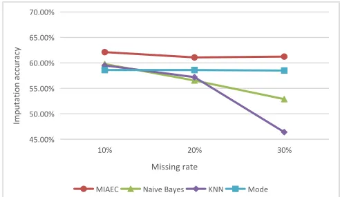
The work in [19] also uses the dataset Adult and gives the imputation algorithm based on Mode, imputation algorithm based on k-Nearest Neighbor experimental results. The experimental results are shown in Figure 5.

45.00% 50.00% 55.00% 60.00% 65.00% 70.00%

10% 20% 30%

Impu

ta

tion ac

cur

ac

y

Missing rate

MIAEC Naive Bayes KNN Mode

Figure 5. The imputation accuracy of missing data under different algorithms

It can be seen from the experimental results that the imputation accuracy of MIAEC is better than that of other algorithms. Imputation algorithm based on Naive Bayes in the low missing rate conditions can play a very good effect, but with the increase of the missing rate, the imputation accuracy will be decreased significantly. The imputation algorithm based on Mode is better in the anti-miss rate, that is, with the increase of the missing rate, the imputation accuracy of the algorithm will not be greatly reduced. The Imputation algorithm based on k-Nearest Neighbor is poor in anti - miss rate, and the accuracy of imputation will decrease sharply with the increase of missing rate.

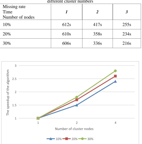
This experiment is to test the distributed parallelism of the algorithm, the algorithm is based on Hadoop platform to implement its Map-Reduce. We test the speedup of the algorithm on the generated data.

Table 1. Algorithm execution time at different missing rate and different cluster numbers

Missing rate Time

Number of nodes

1 2 3

10% 612s 417s 255s

20% 610s 358s 234s

30% 606s 336s 216s

1 1.5 2 2.5 3

1 2 4

The s

peedup

o

f t

he alg

o

rithm

Number of cluster nodes

10% 20% 30%

Figure5. Speedup of the algorithm under different missing rate dataset and different node numbers

V. CONCLUSION

The problem of data loss has caused many difficulties in data mining, especially in the large-scale dataset, the data loss becomes an important factor affecting the quality of data. The processing of missing data has become a very important step in the process of data preprocessing. In this work, we use the evidence chain to predict the value of missing data and estimate the missing value by using the set of combinations of missing attribute values. In order to make the algorithm applicable to large data processing, this algorithm combined with a Map-Reduce framework to achieve the parallel processing of imputation missing data. Experimental results show that the algorithm has high imputation accuracy of missing data, and the imputation accuracy is still better with the increase in missing rate. It does not fluctuate greatly with the position of missing data, and can be applied to the distributed computing environment, and can achieve the ideal algorithm to speed up and so on.

But this algorithm is mainly for the discrete missing data, has some limitations. In addition, since the main computation time of the algorithm lies in the choice of dataset attribute combination, when the dataset attribute dimension increases, the time consumption of the algorithm will increase rapidly. In the future research, we will focus on the imputation algorithm of missing values in the case of continuous data loss and the data reduction method of large data.

ACKNOWLEDGEMENT

This work was partly supported by the Planned Science and Technology Project of Hunan Province, China (2016JC2010).

REFERENCES

[1] D. Bachlechner and T. Leimbach, "Big data challenges: Impact, potential responses, and research needs," 2016 IEEE International Conference on Emerging Technologies and Innovative Business Practices for the Transformation of Societies (EmergiTech), Mauritius, 2016, pp. 257-264.

[2] S. Thirukumaran and A. Sumathi, "Improving accuracy rate of imputation of missing data using classifier methods," 2016 10th International Conference on Intelligent Systems and Control (ISCO), Coimbatore, India, 2016, pp. 1-7.

[3] R.K. Pearson, "The problem of disguised missing data," Acm Sigkdd Explorations Newsletter, vol. 8, no. 1, pp. 83-92, 2006. [4] C. Zhang, Q. Yang and B. Liu, "Guest Editors' Introduction:

Special Section on Intelligent Data Preparation," in IEEE Transactions on Knowledge and Data Engineering, vol. 17, no. 9, pp. 1163-1165, Sept. 2005.

[5] R.J.A. Little and D.B. Rubin, Statistical "Analysis with Missing Data," 2nd ed, United States of America: Wiley-Interscience, 2002, pp. 200-220.

[6] F.Z. Poleto, J.M. Singer and C.D. Paulino, "Missing data mechanisms and their implications on the analysis of categorical data," Statistics and Computing, vol. 21, no. 1, pp. 31-43 Jan. 2011

[7] X. Zhu, S. Zhang, Z. Jin, Z. Zhang, and Z. Xu, "Missing value estimation for mixed-attribute datasets," Knowledge and Data Engineering, IEEE Transactions on, vol. 23, pp. 110-121, 2011. [8] Y. Qin, S. Zhang, X. Zhu, J. Zhang, and C. Zhang, "Semi-

parametric optimization for missing data imputation," Applied Intelligence, vol. 27, pp. 79-88, 2007.

[9] D.B. Rubin, "Multiple imputation for nonresponse in surveys," Statistical Papers, vol. 31, no. 1, p. 180 ,Dec. 1990 .

[10] M. Ramoni and P. Sebastiani,"Learning Bayesian networks from incomplete databases," in Proceedings of the Thirteenth Conference on Uncertainty in artificial intelligence, 1997, pp. 401-408.

[11] Z. Ghahramani and M. I. Jordan, "Mixture models for learning from incomplete data," Computational Learning Theory and Natural Learning Systems, vol. 4, pp. 67-85, 1997.

[12] U. Dick, P. Haider, and T. Scheffer, "Learning from incomplete data with infinite imputations," in Proceedings of the 25th international conference on Machine learning, 2008, pp. 232-239. [13] J. Han and M. Kamber, "Data Mining Concept and Techniques,"

United States of America: Multiscience Press, pp. 184-205, 2001. [14] Z. Shan, D. Zhao and Y. Xia, "Urban road traffic speed

estimation for missing probe vehicle data based on multiple linear regression model," 16th International IEEE Conference on Intelligent Transportation Systems (ITSC 2013), The Hague, 2013, pp. 118-123.

[15] F. Bashir and Hua-Liang Wei, "Parametric and non-parametric methods to enhance prediction performance in the presence of missing data," System Theory, Control and Computing (ICSTCC), 2015 19th International Conference on, Cheile Gradistei, 2015, pp. 337-342.

[16] A. Karmaker and S. Kwek, "Incorporating an EM-approach for handling missing attribute-values in decision tree induction," Fifth International Conference on Hybrid Intelligent Systems (HIS'05), 2005, pp. 6

[18] M. Zhu and X.B. Cheng, "Iterative KNN imputation based on GRA for missing values in TPLMS," 2015 4th International Conference on Computer Science and Network Technology (ICCSNT), Harbin, China, 2015, pp. 94-99.

[19] J. Han and M. Kamber, "Data Mining Concept and Techniques," 3nd ed, United States of America: Multiscience Press, pp. 226, 2012.

[20] P. Keerin, W. Kurutach and T. Boongoen, "Cluster-based KNN missing value imputation for DNA microarray data," 2012 IEEE International Conference on Systems, Man, and Cybernetics (SMC), Seoul, 2012, pp. 445-450.

[21] L. Jin, H. Wang, S. Huang and H. Gao, "Missing Value Imputation in Big Data Based-on Map-Reduce," Journal of Computer Research & Development, vol. 50, no. s1, pp. 312-321 , 2013,

[22] J.L. Yuan, L. Zhong, G. Yang, M.C. Cheng and J.C. Gu, "Towards Filling and Classification of Incomplete Energy Big Data for Green Data Centers," Chinese Journal of Computers, vol.38, no. 12, pp. 2499-2516, Oct.2015

[23] M. G. Rahman and M. Z. Islam, "iDMI: A novel technique for missing value imputation using a decision tree and expectation-maximization algorithm," Computer and Information Technology (ICCIT), 2013 16th International Conference on, Khulna, 2014, pp. 496-501.