An Exploration of Evolutionary Computation Applied
to Frequency Modulation Audio Synthesis Parameter
Optimisation
Thomas James Mitchell
A thesis submitted in partial fulfilment of the requirements of the University of the West of England, Bristol for the degree of Doctor of Philosophy
Bristol Institute of Technology, Faculty of Environment and Technology, University of the West of England, Bristol
i
Acknowledgments
With so many people to thank who have indirectly contributed to this work I would first like to acknowledge those whose names are not mentioned here: family, friends – if you have ever said ―you‘re still doing that?‖ then you know who you are – I am forever indebted.
I would principally like to thank my director of studies Professor Tony Pipe who has been an endless source of inspiration and confidence from start to finish. Additionally, I would like to thank my other supervisors: Dr David Creasey, Dr Marcus Lynch and Stephen Allen whose contributions have been invaluable, especially in the drafting of this thesis. I would also like to thank Professor Alan Winfield for providing a forceful boot onto the path and also for providing funding in desperate times. I would also like to thank the Engineering and Physical Sciences Research Council for providing me with the opportunity to learn about all this stuff.
Finally, I would also like to express my gratitude to Dr Johnson Abraham, Dr Azarhar Machwe and Bhuvan Sharma for their friendship, company, humour and lengthy discussion on this mission; Professor Ian Parmee for the space; Professor Eduardo
ii
List of Publications
Some of the work in this thesis has also appeared in the following publications:
Mitchell, T. J., and Pipe, A. G. (2005) Convergence Synthesis of Dynamic Frequency Modulation Tones Using an Evolution Strategy. Applications on Evolutionary Computing:
EvoWorkshops. 533-538.
Mitchell, T. J. and Sullivan, C. W. (2005) Frequency Modulation Tone Matching Using a Fuzzy Clustering Evolution Strategy. In: Proceedings of the 118th Convention of the Audio
Engineering Society. Barcelona.
Mitchell, T. and Pipe, A. (2006) A Comparison of Evolution Strategy-based Methods for Frequency Modulated Musical Tone Timbre Matching. In: Proceedings of the 7th
International Conference in Adaptive Computing in Design and Manufacture. Bristol. pp.
167-175.
Mitchel, T.J. and Creasey, D.P. (2007) Evolutionary Sound Matching: A Test
Methodology and Comparative Study. Proceedings of The Sixth International Conference
iii
Abstract
With the ever-increasing complexity of sound synthesisers, there is a growing demand for automated parameter estimation and sound space navigation techniques. This thesis explores the potential for evolutionary computation to automatically map known sound qualities onto the parameters of frequency modulation synthesis. Within this exploration are original contributions in the domain of synthesis parameter estimation and, within the developed system, evolutionary computation, in the form of the evolutionary algorithms that drive the underlying optimisation process. Based upon the requirement for the parameter estimation system to deliver multiple search space solutions, existing
evolutionary algorithmic architectures are augmented to enable niching, while maintaining the strengths of the original algorithms. Two novel evolutionary algorithms are proposed in which cluster analysis is used to identify and maintain species within the evolving
populations. A conventional evolution strategy and cooperative coevolution strategy are defined, with cluster-orientated operators that enable the simultaneous optimisation of multiple search space solutions at distinct optima. A test methodology is developed that enables components of the synthesis matching problem to be identified and isolated, enabling the performance of different optimisation techniques to be compared
quantitatively. A system is consequently developed that evolves sound matches using conventional frequency modulation synthesis models, and the effectiveness of different evolutionary algorithms is assessed and compared in application to both static and time-varying sound matching problems. Performance of the system is then evaluated by
iv
Contents
1 Introduction .……….. 1
1.1 Context ………..……. 2
1.1.1 Evolutionary Optimisation ………. 3
1.1.2 Frequency Modulation Audio Synthesis ……… 4
1.2 Objectives ………... 7
1.3 Contributions ……….. 8
1.4 Methodology ……….... 8
1.5 Thesis Structure ……….. 9
1.6 Implementation ………... 9
2 Background: Evolutionary Computation ……….. 10
2.1 An Introduction to Evolutionary Computation ……….. 10
2.2 The Evolutionary Algorithm ……….. 11
2.3 Canonical Evolutionary Algorithms ………... 14
2.3.1 The Genetic Algorithm ………... 14
2.3.2 Evolution Strategies ……….... 17
2.3.2.1 Recombination ………. 18
2.3.2.2 Genetic Repair ………. 19
2.3.2.3 Mutation ……….. 21
2.3.2.4 Selection ……….. 27
2.4 EA Similarities and Differences ………. 27
2.5 Summary of this Chapter ……… 29
3 Background - Multimodal Optimisation ………... 31
3.1 Multimodal Problem Domains and Preconvergence ……….. 31
3.2 Injecting Diversity ……….. 33
3.3 Appropriate Diversity ………. 35
3.4 Speciation ……….... 35
3.4.1 Non Partition-Based Speciation Methods ………... 36
3.4.1.1 Similarity-Based Selection/Replacement ……….... 36
3.4.1.2 Restricted Tournament selection ………. 38
3.4.2 Fitness Sharing ……….... 38
3.5 Static Partition Speciation Methods ……….... 39
3.5.1 Coarse-Grained Parallel Population Methods - The Island Model ………. 40
3.5.2 Fine-Grained Parallel Population Methods: The Diffusion Model ………. 42
3.5.3 Discussion ………... 43
3.6 Dynamic-Partition Speciation Methods ……….. 44
3.6.1 Cluster-Based Partition Methods ……… 44
3.6.2 Alternative Dynamic-partition Methods ………. 48
3.7 Multimodal Optimisation with Cooperative Coevolution ……….. 48
v
4 A Clustering-Based Niching Evolution Strategy ……….. 51
4.1 The Fuzzy Clustering Evolution Strategy (FCES) ………. 52
4.1.1 Cluster Analysis ……….. 52
4.1.2 Clustering for Niche Identification ………. 53
4.1.2.1 Fuzzy Clustering ……….. 53
4.1.2.2 Partitioning Population Members Using C-Means Fuzzy Clustering ……. 55
4.2 Multiple Solution Clustering Evolution Strategy (CES) ……… 56
4.2.1 Restricted Cluster Selection ………... 57
4.2.2 Hard Clustering ………... 58
4.2.3 New Recombination Operators ………... 60
4.2.4 Cluster Quantity – Selecting a Value for K ...……….. 60
4.3 An Analysis of Performance in Selected Test Environments ………. 61
4.3.1 Experimental Introduction ……….. 61
4.3.1.1 Experimental Set-up ……….... 62
4.3.1.2 Algorithm Structure and Parameters ………... 63
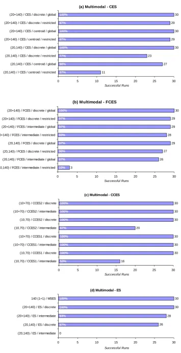
4.3.2 Attribute 1: Global Multimodal Proficiency ………... 65
4.3.2.1 Experiments on the Multimodal Test Function ………... 66
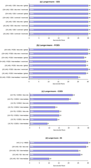
4.3.2.2 Experiments on Langermann's Function ………. 69
4.3.2.3 Experiments on the Maximum of Two Quadratics Function ……….. 71
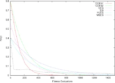
4.3.2.4 Convergence Dynamics ………... 75
4.3.3 Attribute 2: Multiple Solution Proficiency ………. 77
4.3.3.1 Experiments on Himmelblau's Function ………. 79
4.3.3.2 Experiments on the Multimodal Function ………... 81
4.3.3.3 Experiments on the Waves Function ………... 82
4.3.4 Attribute 3: Multidimensional Proficiency ………... 84
4.3.4.1 Experiments on the n-Dimensional Sine Function ……….. 84
4.3.4.2 Experiments on the Multimodal Function ………... 86
4.4 Summary of this Chapter ………... 88
5 Clustering Cooperative Coevolution Strategies – a New Synthesis …………. 89
5.1 Cooperative Coevolutionary Algorithms ……….... 90
5.1.1 Collaboration ………... 91
5.2 CCEAs For Parameter Optimisation ………... 93
5.2.1 Separability, Decomposition and Cross-Subpopulation Epistasis ……….. 93
5.2.2 Relative Overgeneralisation ……….... 94
5.2.3 Modified CCEAs for Single Objective Static Optimisation ………... 95
5.2.4 A Practical Alternative ……….... 97
5.3 Niching in Coevolutionary Algorithms ……….. 98
5.3.1 The Niching Cooperative Coevolutionary Algorithm (NCCEA) ………... 98
5.3.1.1 Collaboration ………... 100
5.3.1.2 Diverse Collaboration ……….. 100
5.3.1.3 Dynamic Linking ………. 101
5.3.1.4 Maintaining Diversity with Exclusive Linkage ………... 102
5.3.2 A Niching Cooperative Coevolutionary Algorithm – The CCCES ……….... 103
vi
5.4 An Analysis of Performance in Selected Test Environments ………. 105
5.4.1 Experiments on Himmelblau's Function ………. 106
5.4.2 Experiments on the Multimodal Function ………... 111
5.4.3 Experiments on the Maximum of Two Quadratics Function ……….. 116
5.5 Convergence Dynamics ……….. 119
5.6 Summary of this Chapter ……… 120
6 The Exploration of FM Parameter Space with Evolutionary Computation ….. 121
6.1 Introduction ………. 122
6.2 Synthesiser Choice ……….. 124
6.3 Frequency Modulation Synthesis ……….... 124
6.3.1 FM Extensions ……… 124
6.3.2 Target Matching with FM Synthesis ………... 126
6.4 Sound Synthesis Applications of Evolutionary Computation ……… 128
6.4.1 Interactive Evolutionary Synthesis ………. 128
6.4.2 Evolutionary Sound Matching ……… 128
6.4.3 A Conspectus of Non-FM Evolutionary Sound Matching Research ……….. 129
6.4.4 Evolutionary Sound Matching with Frequency Modulation Synthesis ……….. 130
6.4.5 New Developments in Evolutionary Sound Matching ……….... 131
6.5 Sound Similarity Measures ………. 133
6.5.1 Content-Based Analysis ……….. 133
6.5.2 Spectrum Error ……….... 135
6.4.3 Windowed Relative Spectrum Error ………... 137
6.4.4 Perceptual Error ………... 139
6.5 Summary of this Chapter ……… 140
7 Experiments in Evolutionary Sound Matching with FM Synthesis ………….. 141
7.1 Evolutionary FM Matching System ……….... 142
7.1.1 FM Synthesis Parameter Ranges ………. 145
7.2 EA Representation ……….. 145
7.3 Evolutionary Matching Synthesis Procedure ……….. 146
7.4 Contrived Sound Matching – An Experimental Test Method …….………... 149
7.5 An Analysis of Evolutionary FM Synthesis Sound Matching Performance ……….. 150
7.6 A Performance Analysis of Evolutionary Static Tone Matching ………... 152
7.6.1 Experiments with Static Tone Contrived Targets ………... 153
7.6.1.1 Contrived Matching with Single Simple FM ……….. 154
7.6.1.2 Contrived Matching with Double Simple FM ………. 157
7.6.1.3 Contrived Matching with Triple Simple FM ………... 159
7.6.2 Experiments with Static Tone Non-Contrived Targets ………... 162
7.6.2.1 Evolutionary Synthesis Matching of Additive-Subtractive Synthesis Tones ………... 163
7.6.2.2 Evolutionary Synthesis Matching of Acoustic Instrument Tones ………... 167
7.7 A Performance Analysis of Evolutionary Time-Varying Matching ………... 171
7.7.1 Experiments with Time-Varying Contrived Targets ………... 171
7.7.1.1 Contrived Matching with Time-Varying Single Simple FM ………. 172
vii
7.7.1.3 Contrived Matching with Time-Varying Triple Simple FM ……….. 176
7.7.1.4 Time Waveform and Frequency Spectrogram Plots with Contrived Targets ………. 177
7.7.2 Experiments with Time-Varying Acoustic Targets ……… 179
7.7.2.1 Time Waveform and Frequency Spectrogram Plots with Non-Contrived Targets ………. 182
7.8 Summary of this Chapter ……… 188
8 Listening Tests ……….. 190
8.1 Introduction ………. 190
8.2 Listening Panel and Test Conditions ……….. 191
8.3 Listening Test One – Similarity Ranking ………...……….... 192
8.3.1 Test Interface and Instructions ……….... 193
8.3.2 Results and Discussion ……….... 195
8.4 Listening Test Two – General Sound Simulations ………...…….. 197
8.4.1 Test Interface and Instructions ……….... 197
8.4.2 Results and Discussion ……….... 201
8.4.2.1 Piano ……….... 201
8.4.2.2 Trumpet ………... 203
8.4.2.3 Violin ………... 205
8.4.2.4 Cymbal ……….... 207
8.5 Chapter Summary and Conclusions ……….... 208
9 Conclusions and Further Work ………. 210
9.1 Thesis Summary and Conclusions ……….. 210
9.2 Contributions ………..……… 213
9.3 Future Work ……….... 215
References ………. 219
viii
List of figures
1.1: Simple FM Model ………... 4
1.2: FM spectrum plots with increasing modulation index, adapted from Chowning (1973) ………... 5
1.3: Bessel functions of the first kind and order n ………. 6
2.1: The evolutionary model ……….. 12
2.2: Canonical GA pseudocode .………. 15
2.3: Multi-membered ES pseudocode ..……….. 18
2.4: Two-dimensional probability isolines of (a) isotropic, (b) ellipsoidal and (c) rotated ellipsoidal mutation ……….. 22
3.1: Island model ……… 40
3.2: Meta-ES ……….. 42
3.3: Fine-grained architecture ……… 43
3.4: Niche identification technique ……… 46
3.5: Cooperative coevolution architecture ………. 49
4.1: FCES pseudocode …….……….. 52
4.2: Pseudocode for the fuzzy centroid optimisation procedure ….………... 54
4.3: Hard cluster centroid optimisation procedure ………. 58
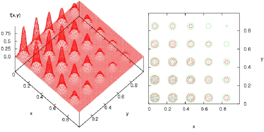
4.4: Multimodal landscape and contour plot ……….. 66
4.5: Results from experiments with the multimodal function .….……….. 67
4.6: Langermans Function with contour plot ………. 69
4.7: Results from experiments with Langermann‘s function ………. 70
4.8: Maximum of two quadratics function with contour plot ……… 72
4.9: Results from experiments with Maximum of Two Quadratics function ……… 73
4.10: Multimodal function convergence dynamics ……….. 76
4.11: Langermann's function convergence dynamics ……….. 76
4.12: Maximum of Two Quadratics function convergence dynamics ………. 77
4.13: Himmelblau's function landscape and contour plot ……… 79
4.14: Mean and 95% confidence intervals for Optima and MPR results on Himmelblau's function ………….. 80
4.15: Mean and 95% confidence intervals for Optima and MPR results on the multimodal function ………… 82
4.16: Waves function landscape and contour plot ………... 83
4.17: Mean and 95% confidence intervals for Optima and MPR results on the waves function ……… 83
4.18: Two-dimentional sine function landscape and contour plot ………... 85
4.19: Mean and 95% confidence intervals for Optima and MPR results on the n-dimensional sine function ……….. 86
4.20: Mean and 95% confidence intervals for Optima and Best solution results on the multimodal function ……….. 87
5.1: Two population NCCEA ……… 99
5.2: NCCEA showing different linkage arrangement ……… 101
5.3: NCCEA with common linkage ………... 102
5.4: NCCEA pseudocode …..………. 103
5.5: Mean and 95% confidence intervals for Total results on Himmelblau‘s function ……….. 107
5.6: Best response curves for the Himmelblau function ……… 108
5.7: Maximum fitness curve for x dimension of Himmelblau‘s function ...……… 110
5.8: Mean and 95% confidence intervals for Total results on Himmelblau‘s function ………. 111
ix
5.10: Mean and 95% confidence intervals for Sum results on the multimodal function ………. 113
5.11: Contour plot of the multimodal function indicating final CCCES solutions ……….. 114
5.12: Mean and 95% confidence intervals for Optima and Sum results on the multimodal function ………… 115
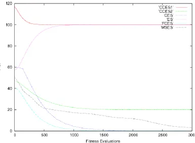
5.13: Convergence trajectories for all algorithms when applied to the MTQ function with discrete recombination ………. 119
6.1: Control to synthesis mapping via intermediate representation ………... 123
6.2: Parallel Simple FM model ……….. 126
6.3: Simple FM landscapes with contrived target at fc = 1760Hz, fm = 1760Hz, I = 4.0 and A = 1.0 produced by the Zero Crossing fitness function (a), and Centroid function (b) ………. 134
6.4: Relative spectral error landscape with contrived target at fc = 1760Hz, fm = 1760Hz, I = 4.0 and A = 1.0 ………. 136
6.5: Frequency spectra of three FM tones ……….. 136
6.6: Equivalent windowed relative squared error landscape with contrived target at fc = 1760Hz, fm = 1760Hz, I = 4.0 and A = 1. 0 ……….. 138
7.1: (a) single, (b) double and (c) triple parallel simple FM arrangements ………... 142
7.2: (a) single, (b) double and (c) triple parallel time-varying simple FM arrangements ……….. 143
7.3: adsr envelope generator ……….. 144
7.4: Evolutionary sound matching model ……….. 146
7.5: Mean and 95% confidence intervals for Average and Remaining error results when matching Single Simple FM contrived tones ………. 154
7.6: Convergence plot for the CCCES and CES ……… 157
7.7: Mean and 95% confidence intervals for Average and Remaining error results when matching Double Simple FM contrived tones ………... 158
7.8: Mean and 95% confidence intervals for Average and Remaining error results when matching Triple Simple FM contrived tones ………. 160
7.9: Static triple FM target (top) and corresponding CES match (bottom) ………... 161
7.10: Static triple FM target and corresponding CES match with log amplitude scale ………... 161
7.11: Unfiltered additive synthesis tone ………... 163
7.12: Additive-subtractive target tone synthesis model ………... 164
7.13: Additive-subtractive target tone spectra ………. 165
7.14: Mean and 95% confidence intervals for error when matching additive-subtractive target tones ... 166
7.15: Acoustic target spectra ……… 168
7.16: Mean and 95% confidence intervals for error when matching acoustic target tones ………... 169
7.17: Muted trumpet tone (top), and corresponding match (bottom) ……….. 170
7.18: Muted trumpet tone and corresponding match with log amplitude ……… 170
7.19: Mean and 95% confidence intervals for Average and Remaining error results when matching time-varying single simple FM contrived sounds ………... 173
7.20: Mean and 95% confidence intervals for Average and Remaining error results when matching time-varying double simple FM contrived sounds ……….. 175
7.21: Mean and 95% confidence intervals for Average and Remaining error results when matching time-varying triple simple FM contrived sounds ……… 176
7.22: Contrived time-varying triple simple FM target and CCES evolved match ………... 178
7.23: Mean and 95% confidence intervals for error when matching acoustic time-varying sounds …………... 180
7.24: Mean and 95% confidence intervals for error when matching an acoustic time-varying oboe sound …... 182
7.25: Oboe target sound and time-varying triple simple FM match evolved by CCCES ……… 183
x 7.27: FM oboe simulation, isolated time domain waveform produced by simple FM element 1 (top), element
2 (middle) and element 3 (bottom) ………. 185
7.28: FM oboe simulation, isolated frequency spectrograms produced by simple FM element 1 (top), element 2 (middle) and element 3 (bottom) ………... 186
7.29: FM oboe simulation, isolated long-term average frequency spectrum produced by simple FM element 1 (top), element 2 (middle) and element 3 (bottom) ……….. 187
7.30: Long-term average frequency spectrum for triple simple FM oboe simulation (top) and original oboe sound (bottom) ……… 188
8.1: Example target sound and five matches with increasing relative spectral error ………. 192
8.2: Listening test 1 interface .……… 193
8.3: Listening test 1instruction sheet ………. 194
8.4: Tone 3 target (top), match 1(middle) analytically ranked 2nd perceptually ranked 3rd, match 2 (bottom) analytically ranked 3rd perceptually ranked 2nd ………. 196
8.5: Listening test 2 interface ………. 197
8.6a: Listening test 2 instruction sheet 1 ………. 198
8.6b: Listening test 2 instruction sheet 2 .……… 199
8.6c: Listening test 2 instruction sheet 3 ………. 200
8.7: Piano target and matched sound time and frequency plots ………. 201
8.8: Trumpet target and matched sound time and frequency plots ………...………. 204
8.9: Violin target and matched sound time and frequency plots ……… 206
xi
List of Tables
4.1: MTQ function parameters ……… 72
4.2: Algorithmic variations for convergence comparison ………... 75
4.3: Multiple solution results of experiments on Himmelblau‘s function ………... 80
4.4: Multiple Solution results of experiments on the multimodal function ………... 81
4.5: Multiple Solution results of experiments on the waves Function ……… 83
4.6: Multiple Solution results of experiments on the n-dimensional sine function ………... 85
4.7: Multiple Solution results of experiments on the multimodal function ……….... 87
5.1: Results of CCCES applied to Himmelblau‘s function ………. 107
5.2: Results of CCCES applied to Himmelblau‘s function with increased cluster quantity ………... 110
5.3: Results of CCCES applied to the multimodal function ………... 112
5.4: Results of CCCES applied to the n-dimensional multimodal function ……… 115
5.5: Results of CCES (various) and CCCES applied to the MTQ function ……… 117
5.6: Results of CCCES applied to the MTQ2 function ……… 118
7.1: Synthesis parameter summary ……….. 145
7.2: Problem space dimensionality summary ……….. 145
7.3: Results when matching Single Simple FM contrived tones ………. 154
7.4: Top 10 multiple solutions delivered by the CES for a contrived match ……….. 156
7.5: 10 multiple solutions delivered by the CCCES for a contrived match ……… 156
7.6: Results when matching Double Simple FM contrived tones ………... 158
7.7: Results when matching Triple Simple FM contrived tones ………. 159
7.8: Top 10 multiple solutions delivered by the CES for a contrived match ……….. 162
7.9: Additive-subtractive target tone specifications ……… 164
7.10: Additive-subtractive target tone results ………... 166
7.11: Acoustic target fundamental frequencies ………. 167
7.12: Acoustic target tone matching results ……….. 168
7.13: Results when matching time-varying single simple FM contrived sounds ……….. 172
7.14: Results when matching time-varying double simple FM contrived sounds ……… 174
7.15: Results when matching time-varying triple simple FM contrived sounds ………... 176
7.16: Acoustic target fundamental frequencies ………. 179
7.17: Acoustic target time-varying matching results ……… 180
7.18: Oboe matching results ……….. 182
8.1: Listening test one correlation and reliability results ……… 195
8.2: Piano semantic differential results ………... 203
8.3: Trumpet semantic differential results ………... 205
8.4: Violin semantic differential results ……….. 206
Chapter 1
Introduction
There is no doubt that modern technology has had a profound effect on the structure, form and performance of music. Powerful and inexpensive general-purpose computers have made electronic musical apparatus widely available to amateur and professional composers alike. The audio synthesiser has, and continues to play an important role in the
To experimental musicians lacking this technical prerequisite, the synthesiser interface can present an obstacle between artistic ideas and their expression. The parameters which are used to shape the sound character are specific to the particular synthesis architecture being employed, and rarely relate to sound in human terms. Consequently, there is a complex mapping between the dimensions of a synthesis parameter (or control) space, and the perceived sound character (or timbre) space. This can often result in an unintuitive synthesiser interface which is concerned with scientific process rather than artistic creativity.
Manufacturers attempt to sidestep this issue by providing a database of parameter settings that enable users to select from a wide range of pre-programmed sounds, known as presets. However, presets only provide access to a limited subspace of the complete synthesis sound space. If it were possible to relate the parameters of a synthesiser more directly to the user‘s intuitive understating of timbre, synthesiser control could become more transparently about sound creation rather than computer programming. The first step to achieving this is the development of a process which is able to map known sound qualities onto sound synthesis parameters. This requires a technique that can efficiently search a synthesis parameter space to identify configurations which achieve specific auricular characteristics. This thesis examines the use of evolutionary computation to do just this, and documents a series of experiments in which evolutionary algorithms are applied to the problem domain of sound matching with frequency modulation (FM) synthesis.
1.1 Context
1.1.1
Evolutionary Optimisation
Artificial models of evolution have been shown to offer many advantages over more traditional optimisation techniques. For example, as evolutionary search is guided by a means of directed stochastic search, high-performance solutions are located more directly than purely random methods (Monte-Carlo search), and more efficiently than enumeration-based methods (brute force search). Maintenance of an advancing population ensures that evolutionary models are less susceptible to becoming trapped within local optima than calculus-based methods (Hill-Climbing), without the need for detailed a priori domain-specific knowledge.
Despite these strengths, evolutionary optimisation is not without weaknesses; in certain applications problems can arise. This thesis is concerned with a class of problem in which multiple distinct high fitness optima may be found within the problem space: the so-called
multimodal problem. The primary reason standard evolutionary algorithms struggle within
these environments is inherent in their fundamental architecture. The model combines stochastic search operators, to explore the problem space, with selective operators, to exploit profitable regions. This mechanism results in a tendency for the algorithm to focus on a single peak, which may be disadvantageous when the application domain is comprised of multiple high-fitness peaks. For the parameter estimation problem explored in this thesis, it is desirable to locate a diversity of solutions and not just one. Optimisation of multiple search space solutions enables a selection of sound matches to be optimised from which the synthesiser user is able to choose. This multiple solution proficiency has
relevance to other application domains in which practitioners may require a variety of design solutions to facilitate better understanding of the underlying problem structure.
1.1.2
Frequency Modulation Audio Synthesis
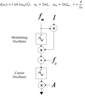
[image:16.595.177.475.240.578.2]FM audio synthesis, presented originally by Chowning (1973), provides a computationally efficient means of creating complex sound timbres, which has seen wide application in commercial systems. In what is termed simple FM, the instantaneous frequency of one sinusoidal oscillator is modulated by another. A diagram of the simple FM model is provided in figure 1.1. and are known as the modulator and carrier frequencies respectively, is the modulation index, and controls the output amplitude. The amplitude function for simple FM is given by the formula:
Figure 1.1: Simple FM model
In equation 1.1, is the modulated carrier output, is the peak output amplitude, and are the carrier and modulator angular frequencies respectively. The modulating oscillator varies the carrier frequency in the range specified by the peak frequency
deviation , which is the product of the modulation index and the modulating frequency . When is assigned a value of zero there is no modulation of the carrier oscillator frequency, and the generated signal equates to a sine wave at frequency . However, when
, frequency partials are generated around the carrier at integer multiples of the modulating frequency as side-bands.
Modulating Oscillator
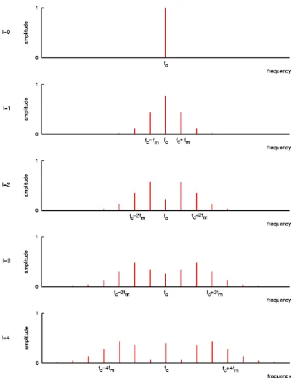
Figure 1.2: FM spectrum plots with increasing modulation index, adapted from Chowning (1973)
As illustrated in figure 1.2, the bandwidth of the modulated signal varies in proportion to the modulation index and modulator frequency. Notice, however, that there is a complex relationship between partial amplitudes and the modulation index I (the envelope of the spectrum is shaped by a non-linear function). The amplitudes of the partials are governed by Bessel functions of the first kind and order , denoted , where the argument to the Bessel function is the modulation index. The Bessel functions are described by the
The Bessel functions for are shown in figure 1.3.
Figure 1.3: Bessel functions of the first kind and order n
The FM signal spectrum is shaped by the functions illustrated above. The amplitude of the partial at frequency is scaled according to the value of , or order function; the amplitude of the first pair of side frequency partials are scaled according to the order function; the second pair of side frequency partials, by the order function; and so forth. The trigonometric expansion of the simpleFM function is given by the expression:
The non-linear relationship between the synthesis parameters and the spectral form of the modulated signal can often complicate the process of sound design with FM. When
parameters are altered by hand it can be difficult to find specific combinations of partials to produce a particular timbre. The sound design process is complicated further by the
coinciding partials: constructive and destructive interference respectively. If the ratio of the carrier to modulating frequency is a rational number, these reflections produce an
arithmetic series of sinusoidal partials with frequencies at integer multiples of a
fundamental frequency: the so-called harmonic spectrum. Conversely, when the ratio is irrational, reflections are positioned between the positive frequency components to produce a non-harmonic spectrum. With so few parameters with which to control such a wide range of timbres, combined with the non-linear effects outlined above, FM has become widely regarded as a difficult synthesis type to control (Kronland-Martinet et al, 2001), (Horner, 2003), (Delprat, 1997), (Payne, 1987). Consequently, a fair proportion of the work in this thesis is concerned with the development of algorithms that are designed to evolve solutions to complex real-world multimodal static optimisation problems. Thus, the fundamental research question that motivates this research is as follows:
Can evolutionary algorithms be created and employed to locate multiple distinct matches of a given target sound, with conventional frequency modulation audio synthesis structures?
1.2 Objectives
To introduce the work set out in the following chapters, the principal objectives which have directed this research are enumerated below.
1. To explore the potential for evolutionary computation as a mechanism for parameter estimation with frequency modulation synthesis.
2. To assess and develop optimisation algorithms suitable for optimising multiple sets of frequency modulation synthesis parameters that approximate a given target sounds.
1.3 Contributions
In satisfying the above objectives the following contributions to knowledge are included in this thesis:
In chapter four, a niching evolutionary algorithm is presented which incorporates k -means clustering into the evolutionary cycle of a conventional evolution strategy to preserve population diversity and enable solutions at multiple distinct optima to be maintained. The algorithm is named the clustering evolution strategy (CES) (Mitchell and Creasey, 2007).
In chapter five, the CES architecture is included into the architecture of the cooperative coevolutionary algorithm, realised as a clustering cooperative coevolution strategy (CCCES), to again enable multiple distinct optima to be maintained while preserving the convergence characteristics of the standard architecture.
In chapter six, a windowed relative spectrum error measure is developed which addresses some of the difficulties associated with comparing sounds using conventional spectrum error measures (Mitchell and Pipe, 2005).
In chapter seven, a contrived testing method is developed which enables the
optimisation component of the matching system to be analysed in isolation without interference from the synthesiser limitations. This enables effectiveness of each optimisation technique to be quantified and compared (Mitchell and Creasey, 2007).
Also in chapter seven, the application of the developed algorithms to six standard and unsimplified continuous frequency modulation synthesisers for matching both static and dynamic sounds (Mitchell and Sullivan, 2005), (Mitchell and Pipe, 2006) and (Mitchell and Creasey, 2007). The developed matching system is then
subjected to perceptual testing in chapter eight.
1.4 Methodology
the parameter estimation problem, algorithm performance is measured according to the matching method described in chapter seven.
1.5 Thesis Structure
The chapters of this thesis have been organised into sections which are largely self-contained. To aid clarity, the algorithmic and application components of the system have been separated, such that chapters two–five concern the development and testing of the evolutionary algorithmic contributions of this thesis in isolation, and chapters six and seven extend their application to the real-world frequency modulation sound matching problem. In reality, the development of the matching system involved interplay between these two components, with evolutionary algorithms developed and tested in application to benchmark test functions, based upon problems that were encountered in the application domain.
Chapters two and three provide a review of evolutionary computation, the major types of evolutionary algorithm and a variety of augmentations to these algorithms which are intended to enhance performance within rugged, multimodal search domains. The evolutionary algorithmic developments of this work are described in chapters four and five, while chapters six and seven provide further review of the frequency modulation sound matching problem and the performance of traditional and developed algorithms within this domain. Chapter eight describes a set of perceptual listening tests with a panel of expert listeners in which the perceived similarity of evolved matches are juxtaposed with their target sounds.
1.6 Implementation
Experimental results provided in this thesis have been produced by applications written by the author in C/C++ using GCC under the GNU/Linux operating system. A number of different synthesis configurations were examined initially using the graphical
Chapter 2
Background: Evolutionary Computation
This chapter provides a brief introduction to the field of evolutionary computation,
including a summary of the general evolutionary model, followed by a review of the major algorithms that embody this field of research.
2.1 An Introduction to Evolutionary Computation
purpose function optimiser by Fogel (1992). Simultaneously, Rechenberg (1965) was working independently on an adaptive optimiser known as the evolution strategy(ES).
Contemporary evolution-inspired function optimisers are descended from one of these three interpretations, which have, since their introduction, been applied to an
ever-increasing number of engineering problems. For a diverse list of applications the reader is directed to Schwefel and Bäck (1997), Bäck et al (1997a) and Rothlauf et al (2005).
Although these three classes of EA are not without difference, each models the processes of evolution to some degree. At an abstract level, evolution can be regarded as the
mechanism by which sophisticated and well adapted biological structures have come to exist: a process of natural selection which emerges when there is a superfluity of genetic material within an environment in which individuals struggle for existence.
Just as a breeder chooses those individuals closest to his desired optimum, and
discards the rest, so the natural environment improves the performance of a species
by eliminating the less effective. Individuals possessing particular adaptations will
survive better, and by virtue of the heritable nature of these adaptations, they will
transmit them to their offspring. Gradually, the adaptations will spread and
improve so that the species will become better suited to the environment which it
inhabits.
Parkin (1979)
2.2 The Evolutionary Algorithm
When the principles of evolution are simulated and used to optimise solutions to
engineering problems, the individuals, referred to in the above quote, are represented by a population of potential solutions. The environment, which is defined by a given objective function, quantifies the relative worth or fitness of each solution. Adaptations are
Figure 2.1: The evolutionary model
This figure illustrates the three core components of the evolutionary model: variation,
selection and the reproductive cycle. Optimisation is achieved by maintaining a population
of solutions, which are alternately subjected to variation and selection. Variation, as already stated, takes the form of recombination and mutation, and represents the birth of new individuals. Before individuals expire, they may be selected for variation based upon their performance within the test environment. The generational cycle repeats until some termination criterion is satisfied: either one or more adequate solutions are engendered, or a generational limit is reached.
To demonstrate how this metaphor of evolution might be applied to optimisation problems, an objective function of the following form is considered:
In this example, the goal of the evolutionary optimiser is to find , a vector of parameters, where , such that the function is minimised (or alternately, maximised):
The first step in applying the evolutionary model is to decide how search points within the objective space are represented. Typically, when optimising parameters of a real-valued objective function, there are two alternatives:
direct, real-valued representation.
mapped, binary-coded representation.
When parameters are represented by real-valued numbers, population members directly represent solutions to the objective function. In other words, each individual contains a complete solution to the function . The ES and EP algorithms both operate directly on the
Variation
object parameters, within what is termed phenotype space. In contrast, traditional GAs employ a binary representation, in which object parameters are encoded into discrete, usually fixed length, bitstrings. These algorithms are said to work in genotype space, and require functions that map individuals between genotype and phenotype space.
Before the reproductive cycle may begin, it is necessary to initialise the system‘s population by generating separate random numbers for each individual. Thereafter, genetic material from the parent population is blended via recombination to generate offspring, which are subsequently varied by means of mutation. Mutation is implemented with the random perturbation of offspring, to introduce chance positive stochastic
variation. Each offspring is then evaluated as a solution to the objective function and assigned a fitness quotient in proportion to its performance. New parents are selected based on their relative fitness, ensuring that high-performing individuals are then chosen to take part in the next round of variation more frequently than low-performing individuals.
A widely accepted viewpoint of the evolutionary process considers selection to encourage the exploitation of high-fitness regions of the solution space, while recombination and mutation facilitate the exploration of new regions which are not currently represented by population. This interplay of exploitation and exploration directs the evolving population towards higher levels of fitness, and thus, evolutionary computation has several advantages over more traditional optimisation methods. For example, enumerative and random-based optimisation techniques are only capable of exploration; consequently the process of optimisation is costly. Hill-climbing-based techniques only exploit and are therefore susceptible to becoming trapped within local optima. The implementation of both search tactics within EAs offers a heuristic optimisation method, which is both robust and efficient.
2.3 Canonical Evolutionary Algorithms
Although the work presented throughout the later chapters of this thesis is largely built upon the theoretical framework of the ES (Beyer, 2001), it is sensible to first consider the general nature of parameter optimisation with EC. This section provides an introduction to GAs and ESs, concluding with a brief summary of their similarities and differences. Further review of EP is not included in this thesis as it is distinguished from the ES and GA, principally by the absence of recombination (Beyer, 2001, p3) (Bäck et al, 1993).
2.3.1
The Genetic Algorithm
The GAwasoriginally developed by Holland to study and model the mechanisms of natural adaptive systems (Holland, 1975). Later, within his doctoral thesis, De Jong (1975) set out the framework for the application of Holland‘s adaptive model to the problem of parameter (function) optimisation. This application formed the precursor to a plethora of GA-based optimisers designed to improve performance when applied to new and
specialised problem domains. This section will provide only a brief summary of the canonical GA; for a more comprehensive introduction with mathematical foundations, see Goldberg (1989) and Whitley (1994).
The canonical genetic algorithm models evolution at the genotypic level, adopting a Boolean representation for the object parameters . The choice of binary-coded
representation is inspired by the way in which biological structures are encoded into the low cardinality alphabet of DNA. Within the GA architecture, individuals are constructed from a single bitstring (chromosome) which is divided into segments (genes) representing each object parameter. To facilitate the optimisation of the function , GAs require functions that map between genotype and phenotype space: and
respectively. Often this mapping procedure is achieved by decoding each binary-represented gene from its integer value, which is then linearly scaled into the range of the corresponding object parameter.
t = 0;
initialise P(t); evaluate P(t); loop begin
P'(t) = select(P(t)); P(t+1) = recombine(P'(t)); P(t+1) = mutate(P(t+1)); evaluate(P(t+1));
t = t + 1; loop end;
Figure 2.2: Canonical GA pseudocode
Where P and P' denote the population and mating pool respectively at time t. Subsequent to initialisation (usually random), each individual of the population is decoded and applied to the objective function to retrieve a value of fitness. In the canonical GA, selection is facilitated probabilistically using the so-called roulette wheel selection mechanism. Each individual is represented by a sector of a notional wheel, sized in proportion to its fitness. A spin of the wheel yields a mating candidate, which is copied into a temporary mating pool (P') in preparation for variation by recombination and mutation.
The recombination operator is termed crossover,and provides the primary source of variation within a GA. The most basic GA recombination technique is known as single-point crossover, which operates by simply concatenating the first part of one parent string with the second part of another; where both the crossover point and the participating parent strings are chosen at random. Crossover is responsible for combining useful segments from the gene pool to form fitter solutions. This concept is otherwise known as the building
block hypothesis, which states that short combinations of highly fit genes (building blocks)
evolve simultaneously throughout the population (implicit parallelism). Well-adapted building blocks are assembled by recombination to create highly fit descendants (Goldberg, 1989). This also relates to Holland‘s schema theory,which states that an exponentially increasing number of trials are allocated to useful building blocks (or
schemata) from one generation to the next (Holland, 1975).
bit position (locus) may be absent or lost from the population which recombination would be unable to recover. To remedy this problem, mutation is applied by randomly inverting bit positions at a low probability, usually around 1% per bit (Schaffer et al, 1989), (Grefenstette, 1986).
Subsequent to fitness evaluation, descendants entirely replace their progenitors to embody the succeeding generation of individuals; this replacement approach is often referred to as
generational. Individuals are then selected from the new population in preparation for
crossover, and the reproductive cycle continues.
GA Performance and Augmentations
The earliest analysis of GA objective function optimisation was performed by De Jong (1975). De Jong compiled a suite of diverse test functions, and introduced two measures to quantify performance:
an on-line measure, to indicate performance within real-world domains, where
emphasis is placed on the rapid location of good results.
an off-line performance measure for simulations in which many function
evaluations may be performed, and the best solution saved for use at the end of a run.
The on-line performance is calculated from the mean average of all fitness evaluations,
while the off-line performance is calculated from the mean average of the best solutions at each generation. De Jong also proposed numerous enhancements and modifications to the canonical GA to provide improved performance when applied to optimise a variety of different problem characteristics. These extensions included:
an elitist strategy, in which the fittest solution at each generation is preserved and copied directly into the next.
an expected value model, with a stable selection scheme to prevent loss of diversity throughout the early stages of evolution.
a generalised crossover operator, to enable multi-point crossover between bitstrings.
a crowding operator, to enhance performance in multimodal environments.
in chapter three. Diversity within the crowding model is maintained by adopting an overlapping (generational) strategy in which offspring replace their progenitors based not on fitness, but similarity in the genotype space.
In the next section of this thesis, the state-of-the-art ES is briefly examined, providing the general framework on which the algorithms presented throughout chapters four and five of this thesis are based.
2.3.2
Evolution Strategies
While EP was being developed in the U.S.A., two engineers at the Technical University of Berlin were independently developing their own evolution-inspired parameter optimisation technique known as the evolutionsstrategie. The earliest ES, developed by Rechenberg (1965), implemented a set of simple rules for the sequential design and analysis of real-world parametric engineering problems.
The ES models the processes of evolution at the phenotypic level. As such, search points are represented directly as n-dimensional vectors of (usually) real-valued object variables
. As well as representing object variables, individuals (denoted ) also include a set of endogenous strategy parameters , as well as a fitness value, equal to its objective function result :
The original two-membered ES (the so-called ES) employs a simple
mutation/selection mechanism, in which a single parent is mutated to produce a single
offspring. If the mutation is found to be profitable the offspring replaces its parent,
otherwise, the offspring is discarded. Later, multi-membered ESs were developed in which populations of parent and offspring individuals are maintained by the algorithm. The two most notable of these population-based ESs were introduced by Schwefel (1981) and constitute:
the strategy, in which parents are varied to produce offspring, and parents of the subsequent generation are selected from all individuals.
the strategy, in which selection is made among only the offspring. Parents are systematically discarded regardless of their fitness value.
t = 0;
initialise Pμ(t);
loop begin
Pλ(t) = recombine(Pμ(t));
Pλ(t) = mutate(Pλ(t));
evaluate(Pλ(t));
P(t+1) = select(Pλ(t) ( + Pμ(t)));
t = t + 1; loop end;
Figure 2.3: Multi-membered ES pseudocode
In this algorithm, Pμ and Pλ denote the parent and offspring populations respectively at
time t. Following the random initialisation of parent individuals, the generational cycle
begins. Genetic information from the parent population is blended via recombination, and then varied by mutation to engender offspring solutions. Thereafter, offspring are evaluated for fitness, and the top individuals are selected deterministically as parents from which the subsequent generation will breed.
2.3.2.1
Recombination
Recombination is the process by which the genetic information is blended to ensure that descendants inherit the characteristics of their ancestors. In the ES, recombination techniques are divisible into two major classes:
intermediate recombination. In which offspring are generated with the mean
average of their parents‘ parameters.
discrete/dominantrecombination. In which offspring parameters (alleles) are
chosen at random from parent candidates1.
Each class has local and global variants. In the former only two parents are married in bisexual recombination, whereas in the latter, all parents partake in multisexual
recombination. Schwefel and Rudolph (1995) extended the ES to include the concept of
variable arity, introducing the exogenous parameter , to indicate the number of parents
participating in the procreation of each descendant. With this generalisation, arity is controlled by the mixing number which may be set to any value in the range . All variants of the ES may then be realised as special cases of the more general
1 This technique is comparable to uniform crossover in the genetic algorithm (Syswerda, 1989),where each
strategy, with indicating a strategy with no recombination and and equating to local and global recombination respectively.
More formally, intermediate recombination amongst parents, is given by:
where represents the object parameter of the parent
, from which the recombinant object parameters , positioned at the centre of mass or centroid of the contributing parents, may be derived. Discrete recombination, on the other hand, is given by:
with chosen randomly anew for all .
Both recombination methods may be applied to the mutation step-sizes in addition to the object parameters .
Eiben and Bäck (1997) empirically investigated the performance of a multi-membered ES in application to a series of test functions, while varying the parameter . The paper
concludes that, in most cases, multisexual recombination of the object variables leads to an increase in performance over asexualrecombination (no recombination), with optimal results often attained when (global recombination).
2.3.2.2
Genetic Repair
The benefit of (intermediate) recombination lies in genetic repair (GR). The effect
of recombination is the extraction of similarities.
Beyer (2001, p222)
When intermediate recombination is applied to a population of parent individuals, recombinants are situated at the centroid of the parent population. Mutation then serves to displace offspring from this centroid position normally at random. Beyer demonstrated that mutants deviate from their origin by a mutation vector which may be decomposed into an
component, in the direction of the optimum, and an component, perpendicular to the direction of the optimum. Deterministic selection of the fittest mutants yields parents endowed with correlated positive components, with relatively uncorrelated
components. By interpreting the component as the harmful effects of mutation (as it lies perpendicular to the beneficial component), the subsequent application of recombination will tend to preserve the useful components of the parents (similarities), while cancelling,
or repairing, their harmful components (differences). In other words, both the beneficial
and harmful effects of mutation are averaged, but selection ensures that the beneficial effects are correlated, while the negative effects are not. Beyer reports that the
component of the calculated centroid is smaller than the mean expected length of a single mutation by a factor of . Moreover, as the harmful component of mutation is reduced by the intermediate strategy, the mutative strength may increase above that which is optimal for a strategy, resulting in a larger improvement step and an overall increase in progress rate.
Interestingly, the genetic repair hypothesis also holds when parents are recombined using the discrete recombination operator. In contrast to the intermediate operator, discrete recombinants are not positioned at the centroid of the parent population. Instead, descendants are constructed from a vector element chosen randomly from the parent population. This procedure is equivalent to randomly sampling the parents‘ genetic material, which is ultimately distributed around a statistical centroid. Thus, recombination can be viewed as a larger (surrogate) mutation from an estimated centroid (Beyer, 1995 and Beyer, 2001).
problems with unknown characteristics. In rugged problem spaces comprising multiple peaks and flat plateaus, recombination and mutation are still beneficial to evolution; however, their benefits cannot be explained by the genetic repair hypothesis alone.
2.3.2.3
Mutation
In contrast to both the GA (in which recombination is widely regarded to be the primary variation operator) and EP (relying upon mutation alone), the ES takes an intermediate position: mutation and recombination are applied with equal importance (Beyer, 2001). However, the mutation operator does provide the primary source of variation, and thus exploration. Recombination works synergistically with mutation, reducing variation error and accelerating progress rates.
Object Parameter Mutation
Mutation is applied to the object parameters of each recombinant with the addition of the mutation vector :
This delivers the mutated object parameters . Each element of the mutation vector is drawn randomly from the standard normal distribution and scaled according to the mutation strength specified by the strategy parameters of the recombinant individual. This mutation scheme ensures that mutative jumps through the search space are:
ordinal, favouring small jumps through the search space over large jumps.
scalable, according to the mutation strength , such that any point within the space
may be reached.
unbiased, ensuring that, on average, mutantsdeviate from their point of origin
isotropically.
The lack of bias in the mutation operator ensures that that there is no deterministic drift without selection.
Variations
sphere, or hypersphere, dependent upon , the problem dimensionality. This is depicted in figure 2.4a (with ).
(a) (b) (c)
Figure 2.4: Two-dimensional probability isolines of (a) isotropic, (b) ellipsoidal and (c) rotated ellipsoidal mutation
With an isotropic mutation mechanism the mutation vector is given by:
As such, each individual within the system contains only one strategy parameter , which offers global control of the mutation step-size for each object parameter.
In many applications it is beneficial to employ an individual step-size parameter for each object vector element, enabling the mutation density function to form an axis parallel ellipse, ellipsoid, or hyper ellipsoid dependent upon (see figure 2.4b). This extension to the mutation operator requires each individual to contain a vector ofendogenous step-size parameters of length . The corresponding mutation vector is then given by:
The most elaborate and general mutation scheme was proposed by Schwefel (1981) and incorporates the concept of correlated mutation angles, in which a rotation matrix enables the density (hyper-)ellipse to adaptively align itself to the topology of the objective function (see figure 2.4c). The corresponding mutation vector is given by:
each individual ( ) and adapted with the step-size parameters . For further reading and implementation details of this generalised self-adaptation mechanism, see (Schwefel, 1981).
When the endogenous strategy parameters ( , and ) are adapted along with the object-variables, optimisation takes place simultaneously in both the object and strategy parameter spaces. This process ensures that high performing solutions are selected for reproduction along with their corresponding strategy parameters, which may go on to yield even stronger solutions throughout subsequent generations.
Strategy Parameter Adaptation
By selecting optimal values for the strategy parameters controlling the mutation strength, the maximum rate of progress can be maintained. The problem then arises as to how the strategy parameters may be continuously adapted throughout the course of evolution. For the ES there are two standard approaches for step-size adaptation: the rule and self-adaptation.
The
Rule
By studying the dynamics of the ES when applied to two differing objective functions, Rechenberg observed that the maximum rate of progress corresponds to a particular value for the probability of a successful mutation (Rechenberg, 1973, as cited in Beyer and Schwefel, 2002). As the mutation step-size tends to zero, the probability of success becomes very high; conversely, as the step-size tends to infinity, the probability of success becomes very low. In order to maintain an optimal rate of progress, the step-size parameter should be adjusted to maintain a probability of success within these two extremes; a range that has become known as the evolution window. This observation led to the derivation of a general rule for the probability of success: mutation step-size adaptation by the rule. Successful mutations are measured over several generations (often equal to the dimensionality of the problem) and if the probability of a successful mutation is found to be below , the mutation step-size is decreased. A recommended factor for the multiplicative/multiplicative inverse adaptation of the step-size parameter by the rule is 0.85 (Schwefel, 1995).
the rule may only be applied when all object parameters are controlled by a global mutation step-size parameter (isotropic mutation).
the rule is only accurate for the two-membered ES.
the rule is only accurate for certain landscape characteristics.
Schwefel (1987) subsequently introduced a more flexible adaptation scheme termed
self-adaptative mutation.
Self-Adaptation
In the self-adaptive mutation scheme, evolutionary search takes place simultaneously in both the object and strategy space. It is assumed implicitly that optimal step-sizes result in fitter descendants and thus will be selected more frequently than non-optimal step-sizes. This adaptation scheme has now become the standard modus operandi for the state-of-the-art ES.
In the self-adaptive method, a vector of step-size parameters is included within each population individual, with the object parameters . Each element of the step-size vector specifies a unique mutation strength for each object parameter, thus facilitating the axis parallel ellipsoidal mutation scheme illustrated in figure 2.4b. To maintain optimal rates of progress, the mutation step-sizes must themselves be adapted along with the object
parameters, by means of recombination and mutation.
Step-Size Recombination
Recombination of the step lengths is considered to be essential for the effective operation of the self-adaptive mechanism (Bäck and Schwefel, 1993). The intermediate and discrete recombination operators, identified above for the variation of object parameters, may be directly applied to vary the step-size parameters.
Step-Size Mutation
To ensure that step-sizes remain positive, the individual step lengths of the vector are mutated by a multiplicative, rather than additive process (as is case for mutation of the object parameters). The principles derived for the mutation of object-variables also apply for the mutation of the strategy parameters. For example, mutations to the object
parameters should be ordinal, scalable and unbiased. However, as mutations are applied multiplicatively they should be drawn from a random number source with expectation 1.0. For this reason the log-normal update rule is applied to the step-size vector as follows:
with and . Schwefel and Rudolph (1995)
recommend setting the learning parameters and , according to:
The order in which the evolutionary operators are applied to the object and strategy parameters is also an important factor in the successful application of self-adaptation. The step-size parameters should be mutated prior to the object parameters, to ensure that any useful mutative step made in the object space is directly attributed to the accompanying step-size vector. The intention here is that the useful strategy parameters that led to the adaptation of strong object parameters are inherited by descendent individuals to deliver even fitter solutions throughout subsequent generations.
Derandomised Self-Adaptation
Firstly, there is no guarantee that profitable variations in the object parameters will naturally correlate with an equivalent change in the mutation step-size. In other words, it is possible for a small step-size to yield a large parameter variation; if the resulting individual is subsequently selected, the step-size does not reflect the advantageous mutation.
Secondly, the amount of variation in the strategy parameters is the same throughout all generations; therefore, the procedure for adapting the strategy parameters is set to facilitate effective mutation irrespective of the distribution of the population throughout the search/strategy space. Consequently, the adaptive process produces a large enough variation in step-size parameters to ensure an appropriate selection difference between individuals. In smaller populations this level of variation can lead to large fluctuations in the strategy parameters that can impede the
optimisation process.
To ameliorate these problems, Ostermier et al derived a derandomised approach to self-adaptation. In the traditional self-adaptive ES mechanism, object parameters are mutated with the addition of the mutation vector :
The derandomised mutation vector is given by:
where or with equal probability determined for each offspring, and z
is a normally distributed random vector. Derandomised mutative adaptation is then applied to the step-size vector according to:
For effective operation of the mutative self-adaptation mechanism, the strategy is widely regarded to offer superior adaptive properties when compared with the
alternative (Bäck and Schwefel, 1993). This is due to the possibility that a highly-fit offspring is generated with a step-size parameter that is entirely inappropriate for its new location. This may arise when a recombinant with a very large mutation step-size
fortuitously jumps to a distant and highly fit region of the search space. If the offspring is able to pass directly into subsequent generations (elitism), optimization is likely to stagnate as further progress will be thwarted by the originally useful but now unsuitably large step-size. This situation could not arise in the strategy, as the anomalous offspring would expire after transmitting some of its strong genetic material through recombination.
2.3.2.4
Selection
The selection operator in the ES facilitates the drift of the population towards regions of increasing fitness within the parameter space. Selection works in an opposing yet complementary manner to the variation operators and identifies the direction in which search should proceed. As was discussed earlier in this section, selection in the ES is performed deterministically. In the case of the comma (or extinctive strategy), the fittest individuals are chosen from the offspring; whereas in the plus (or
preservative strategy), selection is made amongst both the parent and offspring
populations. Schwefel and Rudolph (1995) established the concept of maximal lifespan with the introduction of the exogenous parameter to indicate the number of generations for which each individual is permitted to survive. The resulting strategy provides a generalisation of the deterministic selection scheme, such that when the ES
presents an instance of the extinctive comma strategy; furthermore, when the resulting ES is equivalent to the preservative plus strategy. The parameter may also be set to any intermediary value in between these two extremes .
2.4 EA Similarities and Differences
As the research field of evolutionary computation has developed, the boundaries that once existed between distinct classes of EAs have begun to erode. This section aims to
summarise some of the more recent developments that bring these algorithms closer together.
The canonical GA employs binary encoding for the representation of real-valued object variables. While this type of representation models the processes of biological evolution more closely than real-valued representation, encoding the search space into discrete intervals for binary representation can introduce harmful side effects, which may in turn increase the complexity of the search space (Bäck et al, 1997b). When continuous parameters are represented by bit-strings, there are often large discrepancies (Hamming
cliffs) between the real and encoded parameter spaces. For example, two points might be
separated by only a single bit mutation in the genotype space; however, in phenotype space the same points might be positioned very far apart. This problem may be reduced to some degree by employing a Grey coding, such that all adjacent points in the phenotype space are separated by one bit-shift in the genotype space. However, it is still possible that inversion of a single bit can result in a large transition in object space.
EP and ESs, on the other hand, traditionally represent object parameters with real-valued numbers. This representational distinction between EAs has become blurred since Wright‘s (1991) investigation of real-coded GAs, with phenotypic crossover and (ordinal) mutation operators. This augmentation of the simple GA stimulated a succession of real-coded GA publications that circumvented the inherent precision, range-restriction, and Hamming cliff problems associated with binary-coded representation (Herrera et al, 1998) (Deb and Beyer, 1999). Conversely, ESs may also operate on bitstrings (Beyer, 2001, p3), (Beyer and Schwefel, 2002). An ES has even been adapted to model the neighbourhood
distribution of the Grey-code (Rowe and Hidović, 2004). Consequently, individuals may
be represented directly or mapped via binary-coding in either algorithm.
Schutz (1996) and Bäck et al (2000).
The selection operator may be distinguished from the mutation and recombination
operators as it is entirely independent of the search space structure. As such, any selection operator from one evolutionary algorithm may be easily applied to any other. As was shown earlier, the GA traditionally employs a fitness proportionate probabilistic selection operator. However, tournament selection (Goldberg and Deb, 1991) as well as linear
ranking selection (Baker, 1985)methods are also widely employed. On the other hand, the
ES regularly adopts a deterministic scheme. However, selection operators have also been shared between these two classes: A truncation selectionoperator has been designed and implemented for use within the <