warwick.ac.uk/lib-publications
Original citation:
Ciucu, Florin and Schmitt, Jens (2014) On the catalyzing effect of randomness on the
per-flow throughput in wireless networks. In: IEEE Infocom 2014, IEEE International Conference
on Computer Communications, Toronto, Ontario, 27 Apr - 02 May 2014. Published in: 2014
Proceedings IEEE INFOCOM pp. 2616-2624.
Permanent WRAP URL:
http://wrap.warwick.ac.uk/65277
Copyright and reuse:
The Warwick Research Archive Portal (WRAP) makes this work by researchers of the
University of Warwick available open access under the following conditions. Copyright ©
and all moral rights to the version of the paper presented here belong to the individual
author(s) and/or other copyright owners. To the extent reasonable and practicable the
material made available in WRAP has been checked for eligibility before being made
available.
Copies of full items can be used for personal research or study, educational, or not-for profit
purposes without prior permission or charge. Provided that the authors, title and full
bibliographic details are credited, a hyperlink and/or URL is given for the original metadata
page and the content is not changed in any way.
Publisher’s statement:
“© 2014 IEEE. Personal use of this material is permitted. Permission from IEEE must be
obtained for all other uses, in any current or future media, including reprinting
/republishing this material for advertising or promotional purposes, creating new collective
works, for resale or redistribution to servers or lists, or reuse of any copyrighted component
of this work in other works.”
A note on versions:
The version presented here may differ from the published version or, version of record, if
you wish to cite this item you are advised to consult the publisher’s version. Please see the
‘permanent WRAP url’ above for details on accessing the published version and note that
access may require a subscription.
On the Catalyzing Effect of Randomness on the
Per-Flow Throughput in Wireless Networks
Florin Ciucu
University of Warwick
Jens Schmitt
University of Kaiserslautern
Abstract—This paper investigates the throughput capacity of a flow crossing a multi-hop wireless network, whose geometry is characterized by general randomness laws including Uniform, Poisson, Heavy-Tailed distributions for both the nodes’ densities and the number of hops. The key contribution is to demonstrate
how the per-flow throughput depends on the distribution of 1) the number of nodes Nj inside hops’ interference sets, 2) the
number of hops K, and 3) the degree of spatial correlations.
The randomness in both Nj’s and K is advantageous, i.e., it
can yield larger scalings (as large asΘ(n)) than in non-random
settings. An interesting consequence is that the per-flow capacity can exhibit the opposite behavior to the network capacity, which was shown to suffer from a logarithmic decrease in the presence of randomness. In turn, spatial correlations along the end-to-end path are detrimental by a logarithmic term.
I. INTRODUCTION
A groundbreaking work at the intersection between com-munication networks and information theory is a set of network capacity results obtained by Gupta and Kumar [18]. Under some simplifications at the network layers (e.g., no multi-user coding schemes, or ideal assumptions on power control, rout-ing, and scheduling), those results establish asymptotic scaling laws on the maximal data rates which can be reliably sustained in multi-hop wireless networks. They have further inspired a tremendous research interest and provided fundamental insight into the development of the long desirable functional network information theory (see Andrews et al.[4]).
A major assumption in the network model from [18], which was widely adopted thereafter, is that the geome-try follows a uniform distribution. This assumption implies that the nodes’ interference sets follow the binomial (or its Poisson approximation) distribution. A small set of works considered geometries with specific heterogeneous geometries, which were shown to play a fundamental role in the capac-ity scaling laws (see the Related Work Section). The goal of this paper is to go beyond specific random geometries, by analyzing (throughput) capacity results in networks with general distributions1. To make the analysis manageable, the
paper assumes that network nodes implement the Aloha MAC protocol; the simplicity of the protocol permits the derivation of per-flow capacity results in closed-formand explicitup to the optimization of a single parameter.
We point out that the paper particularly focuses onper-flow capacityresults, rather than the network capacity results which
1In this paper, the notions of throughput and (throughput) capacity, used
interchangeably, explicitly refer to the maximal flows’ throughput achieved in some network, with no coding schemes being considered. The meaning of
capacityemployed herein differs thus from the one in information theory.
are mostly treated in the literature. The advantage of per-flow capacity results is that they determine the network capacity by a summation argument; in contrast, a division argument to compute the per-flow capacity from the network capacity only holds for uniform geometries. Moreover, unlike the majority of existing asymptoticcapacity results—whose practicality is often questioned for small to medium sized networks (Akyildiz and Wang [2], p. 180)—this paper provides non-asymptotic results, e.g., the per-flow capacity in (finite)T time units in a network with (finite)N nodes.
Intuitively, different randomness laws in the geometry yield different (per-flow) capacity results. This paper goes beyond this simple intuition and makes three key contributions:
1) Analyzing the beneficial role of randomness in the network’s geometry on the per-flow capacity. 2) Quantifying the magnitude of the benefit, referred to
as randomness gain, in terms of scaling laws. 3) Providing the “best” distributions maximizing the
randomness gain.
To properly summarize our observations, let us briefly describe the network model; see Section III for the complete description. A flow crosses some end-to-end (e2e) path with
K hops. The interference set of a hop j consists of Nj (interfering) nodes, which is referred to as the hop density; all Nj’s and K can have general distributions. The degree of spatial correlations, denoted by γ, defines the number of consecutive hops with correlated densities; for instance, in the practical scenario when all N1, N2, . . . , NK are statistically correlated, thenγ:=K.
The closed-form expressions of the derived capacity results allow a sensitivity study of the various parameters in the network model, e.g., Nj’s, K, and γ. From this study we collected the following observations:
O1. By scaling N (here a shorthand for Nj’s), the per-flow capacity depends on N’s distribution under a sample-path neighbor-aware probabilities assump-tion. Concretely, nodes should set transmission prob-abilities, explicitly or implicitly, according to the nodes’ densities (transmission probabilities should be roughly proportional to the number of neighbors). With this assumption, different distributions of N
O2. By scaling time, the per-flow capacity is invariant to K. In other words, if the system runs over a sufficiently long time scale, then the per-flow ca-pacity, with the interpretation of a rate, stabilizes and does not depend on the actual number of hops. More interestingly, by simultaneously scaling both time andK, we find that randomness inK has also a fundamental impact on the per-flow capacity (i.e., it changes the order of growth).
O3. The size of the randomness gain can be as large as
O(n)inN and much smaller inK, which indicates that temporal correlations due to N are much more sensitive to randomness than spatial correlations due toK, as an effect of spatial reuse2. Based on specific distributions ofN andK, we find the surprising fact that the randomness gain inKis the logarithm of the randomness gain inN. To clarify its precise meaning, the randomness gain is defined as the relative differ-ence of the per-flow capacities in two scenarios: one in which a network parameter (sayN) is random, and another in which the same parameter N is set to its (non-random) expectationE[N].
O4. By simultaneously scaling time, K, and γ, the per-flow capacity decays logarithmically in γ. The si-multaneous scaling is needed as in 2); otherwise, the impact of spatial correlation vanishes. The observed logarithmic detrimental factor of spatial correlations, is analogous to an existing result characteristic to wired networks: in a tandem of nodes in which exponentially sized packets arrive as a Poisson pro-cess, the e2e delay scales as Θ(nlogn) and not as Θ(n) [7]. The Θ(n) holds under the so-called Kleinrock’s Independence Assumption that packets independently regenerate their sizes at each hop. Without this assumption, the extra logarithmic factor stems from the spatial correlations due to the “very large” packets inducing long delays to packets behind them, and ateachnode. Similarly, in our settings, the logarithmic term arises when spatial correlations span across the entire e2e path.
These insights complement some fundamental existing ones. One is that randomness can have a detrimental role in the network capacity (see Gupta and Kumar [18] or Franceschettiet al.[15]). In contrast, our results show that, in networks with non-uniform geometries, randomness has a ben-eficial role in the per-flow capacity; for a discussion clarifying the apparently contradicting detrimental and beneficial roles of randomness see the end of Section V-A. Another important known fact is that TDMA and CSMA with properly tuned parameters achieve the same capacity (Chauet al.[10]). Such a MAC insensitivity result, however, depends on the assumed uniform geometry. In turn, our results indicate that in a single-hop scenario with non-uniform random geometry, the per-flow capacity is in factsensitiveto the MAC since CSMA implicitly satisfies the sample-path assumption, whereas explicit over-head would be needed for Aloha or TDMA.
2Bytemporal correlationswe mainly refer to dependent events which can
occur simultaneously (i.e., transmissions within the same interference set). By
spatial correlations we mainly refer to dependent events which can occur at different times (i.e., transmissions at two relays whose interference sets share some nodes).
The rest of the paper is organized as follows. First we discuss related work. In Section III, we introduce the network model, and, in Section IV, we introduce the main analytical tools enabling the capacity analysis. In Section V, we first present the main result of the paper, i.e., non-asymptotic bounds on the capacity of a fixed source-destination pair, and then we investigate the capacity’s sensitivity to the random-ness factors in geometry. Brief conclusions are presented in Section VI.
II. RELATEDWORK
Gupta and Kumar [18] analyzed the asymptotic capacity of homogeneous random networks with uniformly distributed nodes, and showed the notoriousΘ 1/√nlogn
scaling law on the per-flow capacity under a specific communication chan-nel model. This law was improved to Θ (1/√n) for another channel model by Franceschetti et al. [15]. Under a mobility model and a two-hop relay model, the per-flow scaling laws were further improved to Θ(1), i.e., the best achievable one, but at the expense of conceivably long delays (Grossglauser and Tse [17]). For a more comprehensive review of related scaling laws see Xue and Kumar [36].
Asymptotic capacities for heterogeneous networks, e.g., not necessarily with uniformly distributed nodes, were derived in special cases. Toumpis [32] considered a logically clustered network in which n sources communicate with nd cluster heads (yet all are uniformly placed), and showed that network capacity degrades in the presence of bottlenecks when 0 < d <0.5. Perevalovet al.[28] considered physically clustered networks, with uniformly placed nodes and clusters of nodes, and showed that network capacity fundamentally depends on the size of the clusters. For some clustered networks, Kulkarni and Viswanath [24] showed that network capacity preserves the scaling law from [18]. For some other specific clustered networks, however, Alfano et al. [3] and Martinaet al. [26] recently showed that the per-flow capacity is fundamentally influenced by the geometry. Similar results have also been reported from simulations by Hoydis et al. [20]. Our paper differs from these works in that it provides per-flow and (non)-asymptotic capacity results for a broad range of random geometries.
Closer to our work, non-asymptotic per-flow capacity bounds were derived in networks with non-randomNj’s and K, and no spatial correlations (i.e., γ = 1) (see Ciucu et al. [12], [11], [13]). This paper extends these results by accounting for general randomness in Nj’s, K, and spatial correlations (i.e.,γ >1).
Our results on the advantageous effect of randomness relate to a “folk theorem” from queueing theory which states that, when the mean inter-arrival (service) time is fixed, the constant inter-arrival (service) time distribution minimizes queueing metrics such as average waiting time. Such results were proven for renewal processes (Rogozin [29]) and also for more general arrival processes with exponential service times (Hajek [19] and Humblet [21]). Moreover, our results on the bimodal nature of distributions maximizing the randomness gain agree with parallel results from queueing theory. For instance, bi-modal distributions maximize queue lengths in GI/M/1 queues (Whitt [33]), in G/M/1 queues with bulk arrivals (Lee and Tsitsiklis [25]), or in queues with bulk arrivals and finite buffers (Buˇsi´c et al.[8]).
III. NETWORKMODEL
In this section, we describe the network model and the type of capacity results investigated in this paper.
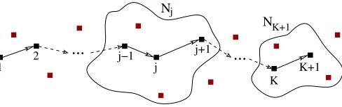
We consider a general network model accounting for three randomness sources, thus significantly generalizing related models. Concretely, we consider the multi-hop random net-work geometry from Fig. 1. Node 1 (the source) transmits to nodeK+1(the destination) using nodes2,3, . . . , Kas relays, where K is a random variable denoting the number of hops. The number of nodes inside the interference set (IS) of nodej, andexcludingnode j, is denoted by the random variableNj, for j = 2,3, . . . , K+ 1; Nj’s are also referred to as nodes’ (hops’) densities. The ISes allow to model arbitrary interfer-ence models and do not rely on geometrical assumptions like disc-based transmission or interference ranges.
One requirement is the existence of an e2e path between the source and the destination. This assumption is motivated by the very goal of the paper, i.e., the derivation of per-flow capacities which requires the flow to be well-defined in terms of an e2e path. If such e2e paths were subject to discontinuities, the derived capacity results would still hold for the transient regimes during which an e2e path exists.
The model further needs knowledge of the distributions of Nj’s and K, which characterize the first two randomness sources. These distributions can be quite general; in fact, the capacity formulae from the main result (see Theorem 1) allow plugging-in any specific distribution law in order to quantify the underlying impact.
Concretely, all Nj’s are finite and identically distributed with density
πn =P(N =n), n= 2, . . . , nmax . (1)
N generically stands for Nj’s. Note that π1 = 0, i.e., the nodes on the e2e path are not isolated, and nmax denotes
the maximum number of nodes inside an IS. The assumption of identically distributed Nj’s is a mild one and mitigates notational complexity.
j
j+1
...
j
N
...
N
K+1 K
K+1
j−1
1 2
Fig. 1. A multi-hop wireless network with a random number ofKhops. The interference set (IS) of nodej contains a random numberNj of nodes. The performance metric of interest is the (non-)asymptotic e2e capacity of node1 transmitting to nodeK+ 1using the nodes2,3, . . . , Kas relays.
For the second randomness source, we assume that the number of hops K is finite, statistically independent of all the Nj’s, and has the density
˜
πk=P(K=k) , k= 1,2, . . . , kmax. (2)
The maximal number of hops is kmax. The independence
assumption simplifies the proof of the main result, i.e., The-orem 1; the proof could also account for the conditional distributionsP(Nj=n|K=k)at the expense, however, of increasing notational complexity. Nevertheless, the indepen-dence assumption betweenK andNj’s is conceivably strong in small networks. Indeed, if nodes set large interfering ranges then the Nj’s are also large and K is small; in turn, if the interfering ranges are small then the Nj’s are also small and K is large. Such correlation effects lessen in large network regimes, whereby our later asymptotic analysis applies.
The third source of randomness in the network model concerns the degree of spatial correlations, i.e., the degree of statistical dependence amongstNj’s. Dealing with all possible combinations and types of such dependencies is clearly an overwhelming task. In our analysis we assume that for each
j = 1,2, . . . , kmax, the r.v. Nj is statistically independent of all Ni’s with i ∈ {j+γ, j+γ+ 1, . . . , kmax}. By the commutativity of the independence relationship between two r.v.’s, Nj is also statistically independent of Ni’s with i ∈
{1,2, . . . , j−γ}.
This particular dependency parameterγ characterizes the maximal number of consecutive ISes for which dependencies (correlations) may exist between the first and the rest. For instance, ifγ= 1then allNj’s are statistically independent; at the other extreme, in a static scenario withkhops,γ=k corre-sponds to dependencies between any pair ofN1, N2, . . . , Nk (this latter scenario is conceivably the most practicalone).
Besides the description of the three randomness sources, the network model requires the specification of the MAC protocol. Concretely, given a slotted time model, the network model requires that all nodes transmit with some probability
p, independently of each other, and from slot to slot. This requirement is immediately satisfied by the slotted-Aloha protocol (Abramson [1]), and implicitly satisfied by 802.11 DCF under an independence assumption from Bianchi [5], in the single-hop case. The assumption from [5], which is commonly adopted in the literature, states that all nodes see the channel in steady state, while the transmission probability
[image:4.595.324.568.103.180.2]also in [5], in Eq. (13)). In a multi-hop case the steady-state assumption becomes however less justifiable, due to the hidden node problem, and further assumptions are needed (Gao et al. [16]). Since we are seeking rigorous capacity results, in order to perform a rigorous analysis of the underlying roles of the three randomness sources, we mainly adopt slotted-Aloha and make side remarks on 802.11 DCF and also on TDMA.
Denoting the transmission from nodei toj by [i→j], a transmission [j → j+ 1] is successful if node j is the only transmitting node inside the IS of nodej+1, in a time slot. As far as data sources are concerned, we assume that the nodes 2,3, . . . , K have infinite buffers and only relay the data from node1 to nodeK+ 1. Also, all the other nodes are saturated, i.e., they always attempt to transmit according to the MAC protocol. This saturation assumption implies that the computed capacity of the path[1→K+1]is conservative from the data-link layer perspective.
The concrete type of capacity investigated in this paper is the per-flow (non-)asymptotic throughput capacity of the transmission[1→K+ 1]. Denote byA(t)the arrival process at node 1 (i.e., counting the data units to be transmitted to nodeK+1). Also, denote byD(t)the corresponding departure process at nodeK+1(i.e., counting the data units arrived from node 1up to timet) . For some fixed violation probabilityε, a probabilistic upper bound on the (e2e throughput) capacity rate is a valueλU
t such that
PD(t)≥λU tt
≤ε . (3)
In turn, a probabilistic lower bound on the capacity rate is a value λL
t such that
PD(t)≤λLtt
≤ε . (4)
We point out that the derived capacity rates λU
t and λLt are obtained in transient (non-asymptotic in the time scale) regimes, whereas the asymptotic results are immediately ob-tained by letting t → ∞. The other non-asymptotic regime is in the nodes’ densities N and number of hops K; again, related asymptotic results follow directly by taking limits.
IV. ANALYTICALTOOLS
In this section, we introduce the modelling tools for the per-flow capacity problem. The main engine behind the derivations in the paper is the framework of the stochastic network calculus, in particular following Fidler [14]. The advantage of the calculus approach is that it considerably simplifies the complexity of modelling a whole network by (logically) reducing it to a single-hop only. It is thus sufficient to model any single-hop scenario from Fig. 1 with sourcejand destinationj+1; the multi-hop model will directly follow from the convolution theorem in the stochastic network calculus.
Let us model an arbitrary single-hop where the source is nodej. For each nodelinside the IS of nodej+1we associate a random processXl(t), wheret represents time. For everyl andt,Xl(t)is a Bernoulli random variable (r.v.) taking value 1 with probabilityp; with abuse of notation, l = 1 refers to the source j. These r.v.’s are mutually i.i.d.in both time and space, and conditioned on the realizations of the number of
nodes/hops (for a parallel analytical framework, dealing with non-necessarily independent increments of Xl(t), e.g., when modelling CSMA/CA besides Aloha, we refer to Ciucu et al. [13]).
Next we introduce the key process for computing the per-flow capacity. This is referred to as the (virtual) interfering process of the transmission[j→j+ 1], and is defined through its increments V(t−1, t) :=V(t)−V(t−1) fort≥1 as
V(t−1, t) = 1−X1(t)
Nj+1
Y
l=2
(1−Xl(t)) . (5)
The initial value is V(0) = 0. We make the important remark thatV(t)does not depend on whether the sourcej is saturated or bursty, since it is defined independently of the arrival process
A(t) at the source. Moreover, as we mentioned earlier, our analysis handles the situation of idle periods characteristic to relay nodes j ≥2, and which are due to internal burstiness: there is nothing to transmit at some slot, and yet the MAC protocol may successfully select the relay node to access the channel. Due to such situations we emphasize the attribute virtual for the processV(t).
Next, we obtain the moment generating function (MGF) and the Laplace transform ofV(t), needed to derive the upper and lower bounds, respectively, from Eqs. (3) and (4). For some parameterθ >0, these transforms are defined as
Mt(θ) =E h
eθV(t)i
andLt(θ) =E h
e−θV(t)i .
The MGF follows from the backwards equations using con-ditioning, and also using the independent increments property ofV(t), i.e.,
Mt+1(θ) = Mt(θ)E h
eθV(1)i
= Mt(θ) X
i
EheθV(1) |N(0) =iiP(N(0) =i)
= Mt(θ) X
i eθq
i+ 1−qiπi .
Therefore, by evaluating the sum,
Mt(θ) =btθ , (6)
where
bθ= 1 +q eθ−1
, q=X
l≥2
qlπl, ql= 1−p(1−p)l−1 ,
and where the πl’s are from Eq. (1). The Laplace transform follows by a sign change, i.e.,
Lt(θ) =bt−θ.
Lemma 1: (SINGLE-HOP (EXACT) SERVICE REPRESEN
-TATION) Consider the interfering processV(t) from Eq. (5). Then the bivariate random process
S(s, t) =t−s−V(s, t) (7)
is an exact stochastic service process for nodeA, i.e.,
D(t) =A∗S(t)a.s. , (8)
for all arrival processes A(t). Here, the symbol ‘∗’ denotes the (min,+) convolution operator defined for all t ≥ 0 as
A∗S(t) := inf0≤s≤t{A(s) +S(s, t)} .
The processS(s, t)quantifies the service received over the link[j→j+ 1]. A key observation is that Eq. (8) holds forall arrival processesA(t). This invariance is instrumental for car-rying out the incoming multi-hop analysis, by circumventing the intrinsically difficult (queueing) problem that the arrival processes at the relay nodes j ≥ 2 are hard to characterize. The processD(t)from Eq. (8) can be also viewed as the output from a variable capacity node (Boudec and Thiran [6]), given the definition of the interfering process V(t) from Eq. (5). Moreover,S(s, s+ 1)can be viewed as the instantaneous per-floweffective capacity, as proposed to model the instantaneous channel capacity by Wu and Negi [34]. In turn, the process
V(s, t)can be viewed as animpairment processas defined by Jiang and Liu [22], p. 72. Having available an exact service process for single-hop transmissions, we can next derive both upper and lower bounds on e2e capacity.
V. END-TO-ENDPER-FLOWCAPACITY
In this section, we first derive the main result of this paper, i.e., a closed-form expression for the per-flow capacity along the e2e path from Fig. 1. Then we investigate its sensitivity to the three randomness sources in the network model: the distribution of the number of neighborsNj’s and the number of hops K, and the dependency parameterγ.
The procedure for getting the upper and lower capacity bounds follows the methodology of the stochastic network calculus (see Boudec and Thiran [6], Chang [9], and Jiang and Liu [22]). First, service processesSj(s, t)for each single-hop transmission[j→j+1],j= 1,2, . . . , K, are constructed as in Eq. (7). These processes are then convolved in the underlying (min,+)-algebra yielding the (network) service process
S(s, t) :=S1∗S2∗. . .∗SK(s, t), (9)
which characterizes the available service (or the per-flow effec-tive capacity in the terminology from Wu and Negi [34]) along the e2e path [1→K+ 1]. Eq. (9) is the convolution theorem from network calculus which reduces the multi-hop analysis to a single-hop analysis. The advantage of the theorem is that it circumvents the difficult problem of modelling input/output processes at intermediate relay nodes, as mentioned earlier.
Theorem 1: (NON-ASYMPTOTIC CAPACITY BOUNDS) Consider the multi-hop network model from Section III with dependency parameter γ. Let ql = 1−p(1 −p)l−1, q = P
l≥2qlπl, andbθ= 1+q eθ−1
for anyθ >0(see Eq. (6)). Then, for some violation probability ε, a probabilistic lower bound on the e2e capacity is for all t≥kmax
λL t = sup
θ>0
1−γ1logθbγθ +logε
tθ −
cK tθ
, (10)
wherecK=Pkkmax=1π˜klog t+k−k−11. The upper bound is
λUt = inf θ>0
1 + 1
γ
logb−γθ
θ −
logε tθ
. (11)
We remark that the asymptotic lower and upper bounds coincide (after using Stirling’s approximation for the factorial in the binomial term, withθ= Θ t−ζ
,0< ζ <1), i.e.,
λ:= lim t→∞λ
L
t = limt→∞λUt = 1−q . (12)
We denote the asymptotic capacity by λ. Theorem 1 general-izes existing non-asymptotic lower-bound results from Ciucuet al. [12], [11], [13] which hold for non-random Nj’s and K, and γ = 1. Moreover, Theorem 1 also provides the corresponding upper bounds. We also point out that the results are explicit up to optimizing afterθ >0.
PROOF. LetPk denote the underlying probability measure conditioned on K =k. Let t ≥0 and the service processes
Sj(s, t)for each transmission[j→j+ 1] forj= 1,2, . . . , k, as in Eq. (7). Applying the e2e service process from Eq. (9), we can write
Pk D(t)≤λLtt
≤ Pk A∗S(t)≤λLtt
= Pk S1∗S2∗. . .∗Sk(t)≤λLtt
,
(13)
because of the saturation conditionA(1) =∞. Lettingu0= 0 anduk=t we can continue above as follows
Pk
inf
0≤u1≤···≤uk−1≤t
k X
j=1
Sj(uj−1, uj)≤λLtt
=Pk inf
0≤u1≤···≤uk−1≤t
k X
j=1
uj−uj−1
−Vj(uj−1, uj)
≤λL tt
!
=Pk
sup 0≤u1≤···≤uk−1≤t
k X
j=1
Vj(uj−1, uj)−
(uj−uj−1)
≥ −λL tt
!
, (14)
where Vj(uj−1, uj) = uj −uj−1 −Sj(uj−1, uj). Next, by applying the Union and Chernoff bounds, we can bound the last term in Eq. (14) by
X
0≤u1≤···≤uk−1≤t
E
k Y
j=1
eθVj(uj−1,uj)
e−θ(
1−λLt)t .
At this point we rearrange the terms in the product in the expectation as
k Y
j=1
eθVj(uj−1,uj)=
γ Y
l=1
Y
i≥0
eθVl+iγ(ul+iγ−1,ul+iγ) . (15)
increments; note the non-overlapping intervals ofVl+iγ’s. With this observation we can bound the last expectation by
γ Y l=1 E Y i≥0
eγθVl+iγ(ul+iγ−1,ul+iγ)
1 γ
= bt γθ
γ1 ,
by using H¨older’s inequality, where bγθ has the expression from the theorem withθreplaced byγθ. Recall also the MGF ofV(t)from Eq. (6).
Collecting terms we obtain
Pk D(t)≤λLtt
≤ X
0≤u1≤···≤uk−1≤t
bt γθ
1γe−θ(1−λLt)t
=
t+k
−1
k−1
bt
γθ
γ1e−θ(1−λLt)t,
where the binomial term is the number of combinations with repetition.
For the upper bound, we recall from Theorem 1 that the service processes Sj(s, t) are exact, and, therefore, the e2e service process from Eq. (9) is exact as well; this property is critical for proving the upper bound. Using again that A(1) =
∞ we can write
Pk D(t)≥λUtt
=Pk A∗S(t)≥λUtt
=Pk S1∗S2∗. . .∗Sk(t)≥λUtt
≤ inf u1≤···≤uk
Pk k X j=1
Sj(uj−1, uj)≥λUtt
. (16)
Foru1≤ · · · ≤uk we can expand the probabilities as
Pk k X j=1
(uj−uj−1−Vj(uj−1, uj))≥λUtt ≤E k Y j=1
e−θVj(uj−1,uj)
eθ(
1−λUt)t,
after using again the Chernoff bound.
At this point, we rearrange the terms in the product as in Eq. (15) and proceed as for the lower bound using H¨older’s inequality first and then the independence property ofVj’s over non-overlapping intervals. We immediately get
Pk D(t)≥λUtt
≤ bt −γθ
1γeθ(1−λUt)t ,
using the Laplace transform from Section IV.
Finally, for some fixed violation probability ε, the lower bound λL
t and the upper bound λUt follow by the change of probability measure P = P
kπ˜kPk, which completes the
proof.
A. Sensitivity to Nj’s
Here, we discuss the capacity’s sensitivity to the distribu-tion of the number of neighbors Nj’s (herein referred to as N). We focus on the asymptotic capacity from Eq. (12), and it is thus sufficient to consider a single-hop transmission.
Let us firstly perform some preliminary calculations. Using Jensen’s inequality we get that
λ=X
l≥2
πlp(1−p)l−1≥p(1−p)E[N]−1 .
The maximum in the last term is attained for p = 1
E[N], and thus λ = Ω (1/E[N]). For the same value of p, and using an upper bound on Jensen’s inequality (see Theorem 1.2 in Simic [31]), we get λ = O(1/E[N]), and therefore the asymptotic capacity scales as
λ= Θ
1
E[N]
. (17)
This scaling also holds in the case of a static network in which
N is a constant, i.e.,P(N 6=E[N]) = 0.
An improved scaling law can be obtained by assuming that, on every sample-path ω, all the nodes are aware of their densities Nω, and set their transmission probabilities to pω=N1ω; this probability is now a random measure. A lower bound on the asymptotic capacity is
λ=X
l≥2
πl 1
l
1−1l
l−1 ≥X l≥2 πl 1 le= 1 eE 1 N ,
after using 1−1
l l−1
≥limn→∞ 1−n1 n−1
= 1
e. In turn, an upper bound is
λ=X
l≥2
πl 1
l
1−1l
l−1
≤X
l≥2
πl 1
l =E
1
N
.
Therefore, with the sample-path neighbor-aware probabili-ties assumption, the asymptotic capacity scales as
λ= Θ
E 1 N . (18)
The same scaling is achieved by an ideal distributed schedul-ing mechanism, such as TDMA (which can be modelled as
Xl(t) = 1ift modN =l−1, andXl(t) = 0otherwise, in Eq. (5)) or by 802.11 DCF, since the transmission probabilities
p implicitly scale asΘ 1
N
(Bianchi [5]). Therefore, CSMA and TDMA networks achieve the same scaling, up to the assumptions discussed in Section III on CSMA; this result was previously shown to hold in the particular case of binomial node densities (i.e., a underlying uniform geometry) and an idealized CSMA model (see Chau et al.[10]).
Inspecting the two scalings from Eqs. (17) and (18), with Jensen’s inequality E[N]E1
N
≥ 1, reveals that the latter is asymptotically bigger. Therefore, the capacity in a ran-dom network with neighbor-aware transmission probabilities is asymptotically bigger than the capacity of a random network with a fixed value for p, or a static network with optimally adjusted p.
The discrepancy between the two scaling laws raises the interesting question on the gain-maximizing distribution of
Dist. πl E[N] EN1
Gain
G-M (20) Θ(n) Θ(1) Θ(n)
Unif. 1
n Θ(n) Θ
logn
n
Θ(logn)
Bnom. nl
(r q)
l
qn Θ (n) Θ 1
n
Θ (1)
Harm. llogκn Θ n
logn
Θ 1 logn
Θ n
log2n
Harm. κ/(nlogn
−l) Θ (n) Θ
1
n
Θ (1)
Hv.tld. κ
l2 Θ (logn) Θ (1) Θ (logn)
Hv.tld. κ
(n−l)2
Θ (n) Θ 1
n
Θ (1)
Sbexp. κ
l3 Θ (1) Θ (1) Θ (1)
Sbexp. κ
(n−l)3
Θ (n) Θ 1
n
Θ (1)
Geom. κal Θ (1) Θ (1) Θ (1)
Geom. κan−l Θ (n) Θ 1
n
Θ (1)
TABLE I. CAPACITY RANDOMNESS GAINS FOR VARIOUS DISTRIBUTIONSπ= (π1, . . . , πn);nIS THE MAXIMUM VALUE OFN.
constant number E[N] of nodes (note that the random and static scenarios are aligned in that the number of nodes are identical, on average). We are thus interested in maximizing the normalized randomness gain
argmax N
Eq. (18)
Eq. (17)= argmaxN E[N]E
1
N
, (19)
subject to the sample-path node-aware probabilities assump-tion. The next theorem provides the soluassump-tion.
Theorem 2: (GAIN-MAXIMIZINGDISTRIB.INEQ. (19)) Denote n=nmax (the maximum value ofN). Then Eq. (19)
is maximized by the distribution
π2=n−E[N]
n−2 , πn=
E[N]−2
n−2 , πi= 0 (i= 1,3, . . . , n−1) (20) when both nandE[N] are fixed.
For the proof see the Appendix. The intuition behind the bimodal distribution is that the increase rate in capacity by lowering the number of neighbors is larger than the decrease rate in capacity by increasing the number of neighbors. Note also that the distribution maximizes not only Eq. (19), but also the capacity when bothn andE[N] are fixed, under the sample-path node-aware probabilities assumption.
Table I illustrates the scaling ofE[N]E1
N
from Eq. (19), for various distributionsπl=P(N =l).κ’s are normalization constants, r = 1−q for the binomial distribution (Bnom.), and 0< a <1 for the geometric distribution (Geom.). There are two versions of harmonic (Harm.), heavy-tailed (Hv.tld.), subexponential (Sbexp.), and geometric distributions, depend-ing on the hops’ density; for instance, row four models a sparse situation with higher densities assigned to smaller number of nodes, whereas row five models the opposite situation.
The reported gain in the last column is relative to the expec-tationE[N]. Note that the gain-maximizing (G-M) distribution from Eq. (20) withE[N] = Θ(n)and the heavy-tailed distribu-tion modelling sparse situadistribu-tions achieve the maximum relative gain, further supporting the observation after Theorem 2. The uniform (Unif.) distribution achieves the same gain Θ(logn) as the first heavy-tailed distribution, but that is relative to an asymptotically larger expected number of nodes, i.e.,Θ(n)vs. Θ(logn).
Summarizing the results, we conclude that the asymptotic (in the time scale) per-flow capacity is fundamentally
influ-enced by randomness in network geometry, but only under the sample-path node-aware probabilities assumption. This assumption requires explicit overhead for both TDMA and Aloha schemes, and it is implicitly satisfied by 802.11 DCF since the nodes’ transmission probabilities arepω= Θ(1/Nω) in steady-state (Bianchi [5]). Similar conclusions can be drawn on the non-asymptotic capacity as well, since the bounds from Eqs. (10) and (11), withθ= Θ t−ζ
[image:8.595.64.288.102.232.2], deviate from Eq. (12) by constant terms depending on the time scale and/or the number of hops. Another interesting observation is that, according to Table I, the randomness gain is non-trivial as long as πldoes not decay faster than κ/l2; an open problem concerns the general distribution ofN for which the gain isω(1).
Let us clarify the apparent contradiction between the above observation that “randomness increases the per-flow capac-ity” and the folk principle that “determinism minimizes the queue” from queueing theory (Humblet [21]) (which agrees in particular with the fact that randomness decreases the network capacity [18]). The reason is that our network model is slightly different than the one from [18], specifically by fixing both the source and the destination and letting the rest be random. Recall that our network model is deliberately tailored to directly study the per-flow rather than the network capacity.
B. Sensitivity to K
Here, we analyze the role of the distribution of the number of hopsK on the lower bound of the non-asymptotic capacity from Eq. (10); as already pointed out, the other capacity results (i.e., the upper bound from Eq. (11) and the asymptotic one from Eq. (12)) are invariant toK. Despite this apparent incom-pleteness (we only analyze the lower bounds), we conjecture that the obtained scaling laws herein hold for upper bounds as well, given the previous observation that the lower bound captures the right scaling in K.
Analyzing the scaling law inKin Eq. (10) yields a trivial result, i.e., Θ(1), since the limit in t must be taken simulta-neously (recall thatt≥kmax in Theorem 1). Informally, note that ift= Θ E[K]1−ζ
, forζ >0, thenλL
t = 0because there are insufficient time slots to carry packets from the source to the destination. To get more interesting results, let us properly scale t= Θ E[K]1+ζ
andγ= Θ(1), for some largeE[K]. Then, the lower boundλL
t decays as
λLt = Ω (−logE[K]) ,
in the case of a static network with a fixed number E[K] of hops. In turn, in the case of a network with a random number of hops K,λL
t decays as
λL
t = Ω (−E[logK]) .
Jensen’s inequality (E[logK] ≤ logE[K]) implies that the lower bound on capacity in a random scenario is asymp-totically bigger than in a static scenario. As in the previous subsection, this discrepancy raises the problem of the gain-maximizing distribution of K which maximizes the random-ness gain, defined here as
argmax K
(logE[K]−E[logK]) . (21)
a difference, and not of a ratio as in Eq. (19). The reason stands in the contribution of K and N to the e2e capacity: the former has an additive effect (i.e., it affects thecumulative throughput), whereas the latter has a multiplicative effect (i.e., it affects the throughput rate).
Theorem 3: (GAIN-MAXIMIZINGDISTRIB.INEQ. (21)) Denote k =kmax (the maximum value ofK). Then Eq. (21)
is maximized by the distribution
˜
π1=
k−E[K]
k−1 , π˜k =
E[K]−1
k−1 , ˜πi= 0 (i6= 1, k) (22) when both kandE[K]are fixed.
The proof is similar to the proof of Theorem 2 and it is omitted.
Similar as in Theorem 2, the intuition for the bimodal distribution is that the rate at which capacity increases by lowering the number of hops is bigger than the rate at which capacity decreases by increasing the number of hops. Note that the distribution from Eq. (22) maximizes not only the randomness gain from Eq. (21) but also the capacity (its lower bound) when both k andE[K] are fixed. Also, note that the randomness gain of the distribution from Eq. (22) can be asymptotically larger than a constant (e.g., Θ (log logk) vs. Θlogk2kwhen E[K] = Θ(logk)).
As far as other distributions are concerned, recall that in the case of the Uniform distribution for the number of neighbors, Table I reports a randomness gain of Θ (logn). In contrast, there is no randomness gain in the case of the Uniform distribution for the number of hops. The reason is that while increasing the number of neighbors has a pronounced effect on capacity, increasing the number of hops has a much more moderate effect due to spatial reuse. This also indicates that spatial correlations are much less sensitive to randomness, as opposed to temporal correlations as observed in the previous subsection. As another closely related example, the first heavy-tailed distribution for N from Table I yields aΘ (logn)gain in Eq. (19). In turn, using the convergence of the series
Pk l=1
logl
l2 , the same heavy-tailed distribution for K has the
gainΘ (log logk)in Eq. (21).
The above example leads us to speculate that for specific distributions of N and K, the (per-flow) capacity gain due to randomness in the number of hops is the logarithm of the capacity gain due to randomness in nodes’ densities.
C. Sensitivity to γ
Here, we briefly investigate the role of the dependency parameterγ on the non-asymptotic capacity.
Note firstly that taking a limit in γ would require taking limits in both E[K] and t. As in the previous subsection, let t = Θ E[K]1+ζ
for some large E[K], but take now
γ = Θ(E[K]) which models a high degree of dependencies amongstNj’s (including the worst-case when all hops’ densi-ties are correlated to each other). Then, the lower bound decays as
λLt = Ω (−logE[K]) , (23)
i.e., the logarithm is the price for assuming a high degree of spatial dependencies in the network. See also Burchard et
al. [7] where the same logarithmic factor is the additional decay on e2e delays (in a Θ(·) sense) in networks with Markovian type of traffic, due to spatial dependencies; recall Item O4 from the Introduction.
Wrapping up, the main observations from this section are summarized in Items O1-O4 from the Introduction. These observations raise an interesting tradeoff between per-flow fair-ness/delay vs. capacity metrics, which has been addressed at the network level in the particular case of uniform geometries (see Grossglauser and Tse [17], Neely and Modiano [27], and Sharma et al. [30]). We believe that a further understanding of this tradeoff at the per-flow level, in networks with general geometries, can inspire distributed network algorithms emu-lating randomness, in order to provide differentiated per-flow services while maintaining a certain level of performance at the network level. More concisely, how could one leverage the randomness in the network geometry, given its advantageous impact on per-flow capacity?
VI. CONCLUSIONS
We have derived closed-form per-flow capacity results, in terms of both upper and lower (non-)asymptotic bounds, on a multi-hop path with a fixed source-destination pair. The key aspect of these results is that they apply to networks withgeneral random geometriesand various degrees of spatial correlations. By exploiting the simple analytical forms of the obtained results, we have quantified the beneficial impact of randomness in geometry on the per-flow capacity metric. In particular, we have shown that different distributions of hops’ densities with normalized averages can lead to gaps in capacity scaling laws as large as Θ(n). We have identified a logarithmic detrimental factor of spatial correlations, and we have further observed a logarithmic relationship between spatial and temporal correlations.
Beyond the intuitively obvious message that randomness matters, this paper strives to communicate how does random-nessquantitativelymatter by analyzing a broad range of distri-butions. The collected observations jointly raise the awareness that the restriction to the widely-adopted uniform geometry model can be quite misleading. Moreover, these observations open the conceivably practical and yet challenging research problem of increasing per-flow capacity by leveraging the randomness in network geometry.
REFERENCES
[1] N. Abramson. The Aloha system: another alternative for computer communications. InProceedings of AFIPS Joint Computer Conferences, pages 281–285, 1970.
[2] I. Akyildiz and X. Wang. Wireless Mesh Networks. Wiley, 2009. [3] G. Alfano, M. Garetto, E. Leonardi, and V. Martina. Capacity scaling
of wireless networks with inhomogeneous node density: Lower bounds.
IEEE/ACM Transactions on Networking, 18(5):1624 –1636, Oct. 2010. [4] J. G. Andrews, N. Jindal, M. Haenggi, R. Berry, S. Jafar, D. Guo, S. Shakkottai, R. Heath, M. Neely, S. Weber, and A. Yener. Rethinking Information Theory for mobile ad hoc networks.IEEE Communications Magazine, 46(12):94–101, Dec. 2008.
[5] G. Bianchi. Performance analysis of the IEEE 802.11 distributed coor-dination function.IEEE Journal on Selected Areas in Communications, 18(3):535–547, Mar. 2000.
[7] A. Burchard, J. Liebeherr, and F. Ciucu. On superlinear scaling of network delays. IEEE/ACM Transactions on Networking, 19(4):1043– 1056, Aug. 2011.
[8] A. Buˇsi´c, J.-M. Fourneau, and N. Pekergin. Worst case analysis of batch arrivals with the increasing convex ordering. In A. Horv´ath and M. Telek, editors, Formal Methods and Stochastic Models for Performance Evaluation, volume 4054 ofLecture Notes in Computer Science, pages 196–210. Springer, 2006.
[9] C.-S. Chang. Performance Guarantees in Communication Networks. Springer Verlag, 2000.
[10] S. Chau, M. Chen, and S. Liew. Capacity of large scale CSMA wireless networks. InACM Mobicom, 2009.
[11] F. Ciucu. On the scaling of non-asymptotic capacity in multi-access networks with bursty traffic. In IEEE International Symposium on Information Theory (ISIT), 2011.
[12] F. Ciucu, O. Hohlfeld, and P. Hui. Non-asymptotic throughput and delay distributions in multi-hop wireless networks. InAllerton Conference on Communications, Control and Computing, 2010.
[13] F. Ciucu, R. Khalili, Y. Jiang, L. Yang, and Y. Cui. Towards a system theoretic approach to wireless network capacity in finite time and space. InIEEE Infocom, 2014.
[14] M. Fidler. An end-to-end probabilistic network calculus with moment generating functions. InIEEE International Workshop on Quality of Service (IWQoS), pages 261–270, 2006.
[15] M. Franceschetti, O. Dousse, D. N. C. Tse, and P. Thiran. Closing the gap in the capacity of wireless networks via percolation theory. IEEE Transactions on Information Theory, 53(3):1009–1018, Mar. 2007. [16] Y. Gao, D.-M. Chiu, and J. C. S. Lui. Determining the end-to-end
throughput capacity in multi-hop networks: methodology and applica-tions. InACM Sigmetrics/Performance, pages 39–50, June 2006. [17] M. Grossglauser and D. N. C. Tse. Mobility increases the capacity
of ad hoc wireless networks. IEEE/ACM Transactions on Networking, 10(4):477–486, Aug. 2002.
[18] P. Gupta and P. R. Kumar. The capacity of wireless networks. IEEE Transactions on Information Theory, 46(2):388–404, Mar. 2000. [19] B. Hajek. The proof of a folk theorem on queuing delay with
applications to routing in networks. Journal of the ACM, 30(4):834– 851, Oct. 1983.
[20] J. Hoydis, M. Petrova, and P. M¨ah¨onen. The effects of topology on the local throughput of ad hoc networks. Ad-Hoc and Sensor Wireless Networks, 7(3-4):337–347, 2009.
[21] P. A. Humblet. Determinism minimizes waiting time in queues. Tech-nical report, MIT Laboratory for Information and Decision Systems, LIDS-P-1207, 1982.
[22] Y. Jiang and Y. Liu. Stochastic Network Calculus. Springer, 2008. [23] L. Kleinrock and F. A. Tobagi. Packet switching in radio channels:
Part I–carrier sense multiple-access modes and their throughput-delay characteristics. IEEE Transactions on Communications, 23(12):1400– 1416, Dec. 1975.
[24] S. Kulkarni and P. Viswanath. A deterministic approach to throughput scaling in wireless networks.IEEE Transactions on Information Theory, 50(6):1041 – 1049, June 2004.
[25] D. C. Lee and J. N. Tsitsiklis. The worst bulk arrival process to a queue. Technical report, MIT Laboratory for Information and Decision Systems, LIDS-P-2116, 1992.
[26] V. Martina, M. Garetto, and E. Leonardi. Capacity scaling of large wireless networks with heterogeneous clusters. Performance Evalua-tion, 67:1203–1218, Nov. 2010.
[27] M. J. Neely and E. Modiano. Capacity and delay tradeoffs for ad hoc mobile networks. IEEE Transactions on Information Theory, 51(6):1917–1937, June 2005.
[28] E. Perevalov, R. S. Blum, and D. Safi. Capacity of clustered ad hoc net-works: How large is “large”? IEEE Transactions on Communications, 54(9):1672–1681, Sept. 2006.
[29] B. Rogozin. Some extremal problems in the theory of mass service.
Theory of Probability & Its Applications, 11(1):144–151, 1966. [30] G. Sharma, R. Mazumdar, and N. B. Shroff. Delay and capacity
trade-offs in mobile ad hoc networks: A global perspective. IEEE/ACM Transactions on Networking, 15(5):981–992, Oct. 2007.
[31] S. Simic. On an upper bound for Jensen’s inequality. Inequalities in Pure and Applied Mathematics, 10(2), 2009.
[32] S. Toumpis. Capacity bounds for three classes of wireless networks: asymmetric, cluster, and hybrid. In ACM MobiHoc, pages 133–144, 2004.
[33] W. Whitt. On approximations for queues, I: Extremal distributions. Technical report, Institute for Systems Research, ISR-TR-1989-37, 1989.
[34] D. Wu and R. Negi. Effective capacity: A wireless link model for support of quality of service. IEEE Transactions on Wireless Communication, 2(4):630–643, July 2003.
[35] M. Xie and M. Haenggi. Towards an end-to-end delay analysis of wireless multihop networks. Ad Hoc Networks, 7(5):849–861, July 2009.
[36] F. Xue and P. R. Kumar. Scaling laws for ad-hoc wireless networks: An information theoretic approach.Foundations and Trends in Networking, 1(2):145–270, July 2006.
[37] K. Zheng, F. Liu, L. Lei, C. Lin, and Y. Jiang. Stochastic performance analysis of a wireless finite-state Markov channel. IEEE Transactions on Wireless Communications, 12(2):782–793, Feb. 2013.
[38] H. Al-Zubaidy, J. Liebeherr, and A. Burchard. A (min,×) network calculus for multi-hop fading channels. InIEEE Infocom, 2013.
APPENDIX
PROOF OFTHEOREM2. According to Eq. (18) we have to solve a linear program with the objective function
max πi
X
i≥2 1
iπi
subject to the constraints
X
i≥1
iπi=m, X
i≥1
πi= 1, πi ≥0 .
Recall that π1 = 0 (there are at least two nodes). Select some πi’s satisfying the above constraints and assume that there exists i ∈ {3, . . . , n−1} such that πi 6= 0. The idea is to appropriately redistribute the entire value of πi to the extremes π2 and πn, and then show that the new distribution increases the objective function.
Letx= n−i
n−2πiand consider the new distributionπ
′ isimilar toπi except for
π′
2=π2+x, π′i= 0, π ′
n =πn+πi−x .
One can check that the redistribution ofπipreserves the mean m. It remains to prove that
1 2π2+
1
iπi+
1
nπn ≤
1
2(π2+x) + 1
n(πn+πi−x) .
By rearranging terms the inequality reduces to i≥2which is true.
One can repeat the above procedures for all i in the set
{3, . . . , n−1} satisfyingπi6= 0, and reduce the initial linear program to
max π2,πn
1
2π2+ 1
nπn
,
subject to the constraints
2π2+nπn =m, π2+πn= 1, π2≥0, πn≥0 .