ISSN: 1816-949X
© Medwell Journals, 2020
Calibration of Industrial Robot Kinematics Based on Results of
Interpolating Error by Shape Function
Thuy Le Thi Thu, Khanh Duong Quoc and Long Pham Thanh
Division of Mechatronics, Faculty of Mechanical Engineering,
Thai Nguyen University of Technology, Street No. 666, 3/2, Tich Luong Ward,
Thai Nguyen City, Thai Nguyen Province, Vietnam
Abstract: The initial accuracy of a robot arm depends not only on the hardware’s manufacturing and assembly quality but also on control strategies. During assembly or regular maintenance, the kinematic accuracy of a robot arm needs to be verified and calibrated to maintain the desired quality. In this study, we present a method to determine and correct the robot kinematic error based on the shape function interpolation technique. Experimental research was applied to aABB robot with six degrees of freedom to verify the correctness of the method. The results indicated that the position errors of the end-effector were significantly reduced. The effectiveness of the proposed interpolation method and combined error compensation algorithm demonstrated that practical application is feasible.
Key words: Calibration, error kinematics, interpolation, shape function, industrial robot, application
INTRODUCTION
Today, robotic arms play an important role in industrial applications. The accuracy of these manipulators should be maintained over time to ensure product quality. As such, many studies have been conducted to improve the calibration and maintain the desired accuracy of robot grippers. These studies are classified into two methods: model-based and modeless. The classical model-based method for robot calibration involves setting up a kinematic model for the robot, measuring positions and orientations of the robot end-effector, identifying its kinematic parameters and compensating its pose errors by modifying its joint angles (Mooring et al., 1991). The advantage of model-based calibration is that a large workspace can be calibrated accurately and all pose errors within the calibrated workspace can be compensated by joint angles (Bai and Wang, 2006). Therefore, a significant amount of research has been performed in this direction. Several recently published studies-such as that by Wang et al. (2012) used genetic algorithms to build mathematically calibrated equations to compensate the kinematic errors cylindrical-coordinate-based manipulator with three Degrees of Freedom (DOF). Ma et al. (2018) conducted modelling and calibration of high-order joint-dependent kinematic errors for industrial robots. The process was performed using high-order Chebyshev polynomials to represent individual error terms and a laser tracker system to acquire the measured data. Laser tracker systems are often used in studies of kinematic error calibration of
series and parallel robots (Abderrahim et al., 2006; Kamali et al., 2016; Sun et al., 2016). Yu and Xi (2018) presented a self-calibration method based on measuring the centers of four spherical calibration targets located around the inspecting system. Their global kinematic model was developed based on a Modified Denavit-Hartenberg (MDH) Model without separating the hand-eye and robot exterior models. The MDH method and Hayati convention were also used by Kong et al. (2018) to calibrate the kinematics and enhance the accuracy of a 3-PRRU parallel manipulator through the effect of error of its universal joints. However, the disadvantage of the model-based method is that an understanding of modelling and identification processes requires advanced knowledge of robot kinematics.
In the modeless method, kinematic modelling and identification steps are not required. The disadvantage is that the accuracy depends on the number of grid points. However because of its simplicity and efficiency, the modeless technique is widely applied in industrial fields. Several researchers have conducted error calibration of robotic arms through this interpolation technique. Liu et al. ( 2018) proposed a trajectory planning technique to minimise the synthetic error of the end-effectors of industrial robots. Kinematic and dynamic models were built using screw theory and Kane equations and subsequently, the end-effector synthesis error was modelled by considering the effect of interpolated algorithms and the flexibility of all joints. The septic polynomial was used to interpolate the via. points in joint space and the PSO algorithm was applied to find the
Kinematic compensation Interpolating the
end-effector error from the shape function Establish
shape functions Experiment
measurements Determining a survey
space and grid points
Determining error Calibrating error
minimum synthesis error. In Bai and Wang (2016), used an Interval Type-2 Fuzzy Error Interpolation method (IT2FEI) to compensate the calibration accuracy of a robot in a 3D workspace. Theirs was compared to other nominal interpolation methods: type-1 fuzzy, trilinear and cubic spline. Meanwhile, Borrmann and Wollnack (2014) used a laser tracker to measure the position and direction of the linear axis. B-spline interpolation was used to model the external axis which allowed for prediction of the linear axis pose. Bai and Wang (2006, 2003a, b, 2004), Bai and Zhuang (2004, 2005), Bai et al. (2008), presented a modeless technique in combination with an online fuzzy interpolation method to calibrate the accuracy of a serial and parallel (Stewart Platform) robot.
MATERIALS AND METHODS
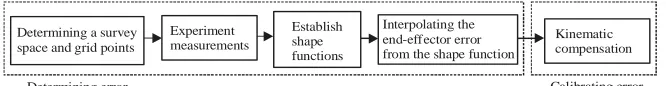
In this study, the researchers present a procedure for determining errors according to the modeless method with shape function interpolation techniques. Calibration is then performed to minimise the kinematic errors of the end-effector of a robot. The general process is described in Fig. 1.
RESULTS AND DISCUSSION
The rest of this study is organized as follows: first, the determination of a robot’s end-effector error is presented as two primary steps: measure the errors at certain poses in the survey space by an experimental measuring system and from those sample poses, establish the shape function interpolation to compute the errors of the entire survey area. The second section, errors. In the third section, the effectiveness of the proposed method is verified on a ABB robot with six DOF (6DOF).The final section outlines the conclusions.
Determining kinematic errors of robot end-effector Basis of determining end-effector errors of robot at sample poses in the workspace: To predict the errors of the robot end-effector in the workspace, several sample poses need to be measured experimentally to find the actual errors. These errors are used as input to construct interpolation functions for predicting the deviations of the gripper at other poses in the survey space.
Manipulators always face objective obstacles such as link parameter errors, clearances in the mechanism’s
connections, wear, thermal effects, flexibility of the links and gear train, gear backlash, encoder resolution errors, errors associated with relating the theoretical robot coordinate frame to the world coordinate frame and control errors (Hayati et al., 1988). Therefore, when controlled to reach the desired pose P (Px, Py, Pz), the tip of the robot will reach the pose with the real coordinate P’ (px±δx, py±δy, pz±δz) in which at various poses throughout the workspace and even at the same pose, the errors (δx, δy, δz) are different. The
manufacturer’s published value for these errors is statistically significant. The errors will increase with the service time of the robot. In performing the study, we used a robot with a software interface designed to be able to read both the coordinates of pose P (Px, Py, Pz) and the
corresponding generalized coordinates P (q1, ...., qn).
In Fig. 2, the coordinate origin O0 of the robot is determined as the center of the top face of a cylindrical cotter pin located in the robot body. When the cylindrical pin is placed in the base of the manipulator, its center is on the first axis of rotation. Therefore, in the kinematic model, the robot arm is at coordinate origin O0.
The purpose of setting this pin is to transfer the virtual origin O0 into a real one, thereby allowing the
camera see and determine its location. Subsequently, the camera software determines the conversion of the coordinate system to convert all observed data through this origin point O0 of the robot.
The two pins are set in a high-precision jig at a distance of d from one another, as shown in Fig. 3. The position and direction relations between them are determined by the transfer matrix:
(1)
0 C
O
0 O C
O *A O
Where, OC is the origin of the reference system attached to the camera.
At this time, there are two independent observation channels:
C Coordinate P (Px, Py, Pz) is the desired pose. It is determined based on the encoders e1, e2,..., en as shown in Fig. 3 and displayed on the interface of the robot
C Real coordinate P’ (px±δx, py±δy, pz±δz) is that
[image:2.612.141.474.652.695.2]determined independently by the camera and transferred to an origin O0 relation according to Eq. 1
Z0
X0
Y0 X0
Z0
Y0 O0
E
F
D NE
C B
NF
ND
A
NA
NB
NC Pi
Z0
Y0
X0
O0 OC
e1
p
d e2
[image:3.612.83.290.91.235.2]e3
[image:3.612.329.524.95.262.2]Fig. 2: Position of basic reference coordinate system on cylindrical cotter pin and position of the pin in the manipulator
Fig. 3: Camera and robot arranged on a specific jig to identify the origin point O0
Comparing these two coordinates will produce the absolute error of the robot end-effector in pose P (δx, δy, δz).
Error prediction with shape function: Data obtained by
direct measurement of the entire workspace have a high time cost and are not suitable for industrial production conditions. As such, we replaced the measured data with interpolated data before error compensation. Accordingly, the error calibration process was accelerated.
In the workspace, a group of sample points are used to form the survey space. These points are referred to as nodes and are associated with other individual points. Once the errors corresponding to each node have been determined through direct measurement, errors at arbitrary positions in the survey space can be interpolated by introducing a suitable interpolation scheme. For this, three-dimensional interpolation is implemented with shape functions.
If there are n nodes, n shape functions will be defined. With the determination of the end-effector error of the robot consisting of six components
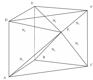
Fig. 4: Influence of sampling points on a survey point through shape function
(three orientation and three position components), to compute the coefficients of the shape functions, the survey space is selected to include six nodes. In this case, the researchers selected the survey space as a triangular prism; i.e., six sampled points will form a six-node brick element.
Suppose the error at survey pose Pi consists of six
components as follows:
(2)
i i i i i i Pi ( x, y, z, x y, z)
Consider the survey space as shown in Fig. 4. In this field, the errors are measured at the vertices of the prism with each vertex corresponding to the six components in Eq. 2.
At pose Pi in the triangular prism, the following
relationships are established:
(3)
(i) (A) (B) (F)
δx = NA.δx + N .Bδx + ... + N .Fδx
...
(i) (A) (B) (F)
δθz = NA.δθz + N .Bδθz + ... + N .Fδθz
Where, are the six(i)x ,y(i),z(i),θ(i)x ,θ(i)y ,θ(i)z
component errors at pose Pi.
NA, NB, NC, ND, NE and NF are the stationary
coefficients of the shape functions that affect the error at pose Pi from the six corresponding nodes and are the
(A) (A) (A) (A) (A) (A) (F) (F) (F) (F) (F) (F) δx ,δy ,δz ,δθx ,δθy ,δθz ,δx ,δy ,δz ,δθx ,δθy ,δθz
are the actual component error values for position and direction (directly measured) of the six corresponding A...F vertices.
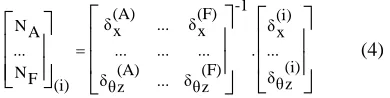
[image:3.612.73.295.118.399.2](4)
-1
(A) (F) (i)
δ ... δ
NA x x δx
... ... ... ... . ... (i) (A) (F)
NF δ ... δ δ
θz (i) θz θz
where in the right-hand side of the equation, the square matrix is the measured error values of the vertices A, …, F and the matrix is the measured error values
T (i) (i)
δx ...δθ z
at the survey pose Pi in the prism, is the
T NA, ..., NF (i)stationary values of six shape functions impacting the errors at pose Pi.
After n survey poses, the result is a set of n sets of stationary values of six shape functions, as follows:
(5)
NA NA NA
... ; ...; ... ; ...; ...
NF NF NF
(1) (i) (n)
Thus, the regression law allows for the determination of the experimental shape function at vertex k as follows:
(1) (i) (n)
(Nk , ..., Nk , ..., Nk )fk(x, y, z)
(k = A, B, C, D, E, F) (6)
At this time, according to Eq. 3, it is possible to calculate explicitly the error at pose Pi having arbitrary coordinates in the survey prism. Subsequently, the interpolated errors at this pose are determined by the shape functions. This procedure greatly reduces the complexity and computational burden associated with direct evaluation of the errors and as will be demonstrated can result in remarkable prediction accuracy (Wang et al., 2002).
Compensation of end-effector error based on results interpolation: As kinematic error is the primary source of inaccuracy in a robot end-effector Weill and Shani (1991) Conrad et al. (2000), it must be sufficiently compensated. The basis of the proposed error compensation method is to control the robot to an alternate pose instead of the desired pose.
The basis of the error compensation method herein is to control the robot to an alternate pose instead of the desired pose. This alternative point is proposed to compensate for kinematic errors that appear when the robot gripper is controlled straight to the desired destination.
Let:
(i) (i) (i) P (x , y , z ,i i i i θx ,θy ,θz )
and
(i) (i) (i) (i) (i) x ±δ , y ±δ , z ±δ ,θ ±δ , t i x i y i z x θx Pi (i) (i) (i) (i)
θy ±δθy ,θz ±δθz
Be the desired coordinate of the manipulator and the actual coordinate recorded by interpolation using the shape function, respectively for the same survey pose (Pi) (Fig. 5). Thus, there exists a deviation of six components between them:
i i i i i i
δP = (±i δx, ±δy, ±δz, ±δθx, ±δθy, ±δθz)
To reduce this error, we propose to replace posepi when solving the inverse kinematic problem with pose Pi,
which is determined from the desired coordinate and its errors as follows:
(7)
(i) (i) (i) (i) (i) x δ , y δ , z δ ,θ δ , ' i x i y i z x θx
Pi (i) (i) (i) (i)
θy δθy ,θz δθz
After resolving the inverse kinematic problem with the destination as Pi instead of Pi, the result will be significantly improved accuracy (Table 1).
Illustrative examples and experimental results:In this
[image:4.612.105.300.100.149.2]section, an experimental survey is presented to verify the proposed theories. The system consists of a 6DOF ABB robot and Cognex 3D-A5005 area scan 3D camera. The kinematic parameters of the robot are shown in Table 2. The camera has an XY resolution of 44 µm, Z resolution of 8 µm and repeatability of 6 µm. In this experiment, the camera was calibrated with a Root Mean Square (RMS) index of 0.005 mm (Fig. 6).
Table 1: D-H link parameter table
Joint i Rz Tz Tx Rx
1 (α1) d1 a1 90E
2 (α2) 0 a2 0
3 (α3) 0 a3 90E
4 (α4) d4 0 -90E
5 (α5) 0 0 90E
6 (α6) d5+d6 0 0
Table 2: Nominal link lengths (mm)
d1 a1 a2 a3 d4 d5+d6
[image:4.612.316.538.607.720.2]E
F
D
A
G
C B
H
[image:5.612.93.283.90.314.2]+Pi
Fig. 5: Kinematic modelling of ABB
Fig. 6: Experimental diagram
Error interpolation by shape function: Assuming the
robot’s operational space in the experiment is a rectangular prism (as shown in Fig. 7), construction of the shape function is performed in each constituent triangular prism-ABCDEF and AGCDHF to predict the end-effector errors.
Interpolation of errors in prism 1-ABCDEF: The
[image:5.612.325.518.99.284.2]survey space is a triangular prism with vertices of six nodes: A, B, C, D, E and F. The experimental process was conducted with 54 grid points in this space. Two data points describing the pose at these points are recorded independently: the nominal pose displayed on the robot controller and the actual one
[image:5.612.75.291.347.526.2]Fig. 7: Survey prism for predicting end-effector errors recorded by the 3D camera. Thesevalues are then compared to acquire the errors at point Pi.
Table 3 shows the nominal and real position values and errors. In the table, a13, a23 and a12 represent 3 values about the orientation cos (x0, z6), cos (y0, z6) and cos (x0, y6) and a14, a24 and a34 are the positions px, py and
pz, respectively.
The set of error values of the six nodes and 54 grid points is used as input to construct the shape functions for predicting the end-effector errors as described in section 2.2. The shape functions in the survey space are determined by an experimental regression in Minitab Software, as follows:
NA = -18.48+0.0675*X+0.0318*Y+0.0219*Z +0.000005*X*X+0.000090*Y*Y+0.000049*Z*Z
-0.000145*X*Y-0.000100*X*Z-0.000094*Y*Z NB = 10.08-0.0307*X-0.0123*Y-0.01576*Z+
0.000016*X*X-0.000091*Y*Y-0.000021*Z*Z +0.000081*X*Y-0.000000*X*Z+0.000095*Y*Z
NC = 12.59-0.0404*X-0.0178*Y-0.02115*Z -0.000025*X*X-0.000015*Y*Y-0.000017*Z*Z +0.000083*X*Y+0.000099*X*Z-0.000002*Y*Z
ND = 13.64-0.0526*X-0.0258*Y-0.02876*Z
+0.000009*X*X-0.000053*Y*Y-0.000037*Z*Z +0.000101*X*Y+0.000101*X*Z+0.000097*Y*Z
NE = -7.76+0.0332*X-0.0000*Y+0.02115*Z
-0.000030*X*X+0.000085*Y*Y+0.000011*Z*Z -0.000065*X*Y-0.000000*X*Z-0.000096*Y*Z NF = -8.94+0.02182*X+0.02405*Y+0.02343*Z +0.000024*X*X-0.000020*Y*Y+0.000014*Z*Z
Table 3: Nominal and real pose values at survey points
Desired position Measured pose Measured pose errors
--- --- ---Point X Y Z a13 a23 a12 a14 a24 a34 δ a13 δ a23 δ a12 δ a14 δ a24 δ a34
Where, NA, NB, NC, ND, NE and NF are the shape
functions describing the error influence from nodes A, B, C, D, E and F, respectively on point Pi with coordinates (X, Y, Z).
Interpolation of errors in prism 2-AGCDHF: The same
process is followed for the second prism to produce the following regression:
NA = 118.1+0.649*X+0.285*Y-1.873*Z
-0.001090*X*X-0.000363*Y*Y+0.003799*Z*Z -0.000605*X*Y+0.000004*X*Z-0.000010*Y*Z
NG = -67.8-0.401*X-0.172*Y+1.1179*Z
+0.000692*X*X+0.000165*Y*Y-0.002284*Z*Z +0.000392*X*Y-0.000044*X*Z+0.000067*Y*Z
NC = -55.1-0.311*X-0.144*Y+0.8996*Z +0.000492*X*X+0.000223*Y*Y-0.001836*Z*Z +0.000294*X*Y+0.000047*X*Z-0.000048*Y*Z
ND = -111.7-0.646*X-0.280*Y+1.830*Z
+0.001055*X*X+0.000317*Y*Y-0.003708*Z*Z +0.000636*X*Y-0.000007*X*Z+0.000007*Y*Z
NH = 67.6+0.434*X+0.167*Y-1.1496*Z -0.000725*X*X-0.000139*Y*Y+0.002350*Z*Z -0.000428*X*Y+0.000042*X*Z-0.000069*Y*Z
NF = 49.4+0.2696*X+0.1407*Y-0.8120*Z
-0.000417*X*X-0.000204*Y*Y+0.001653*Z*Z -0.000280*X*Y-0.000043*X*Z+0.000053*Y*Z
This result is used to predict the end-effector error at any position in the survey space. Because the interpolation is based on directly measured errors, it
includes all component error sources. Hence, the interpolated error values are implicitly the synthesis errors.
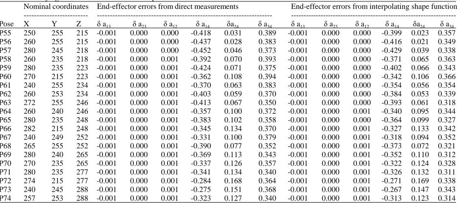
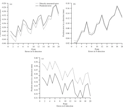
Verification survey: To verify whether the shape
function has been met, we compared the errors at 10 random points in the survey space. Errors were taken from two separate sources: those directly measured and those predicted from shape functions. The deviations are shown in Table 4.
The graph in Fig. 8 shows the correlation between the position deviation of the end-effector measured experimentally and that determined by the shape function in the X, Y and Z directions. In the graphs, the red line represents the error measured experimentally and the blue represents the error interpolated from the shape function. The charts show that the robot end-effector error interpolated from the shape function has a deviation from the experimental measurement in the range from 0-0.035 mm. Thus, the interpolation result can be used to replace the direct measurement results. This saves considerable time and cost for designing, calibrating and determining robot error.
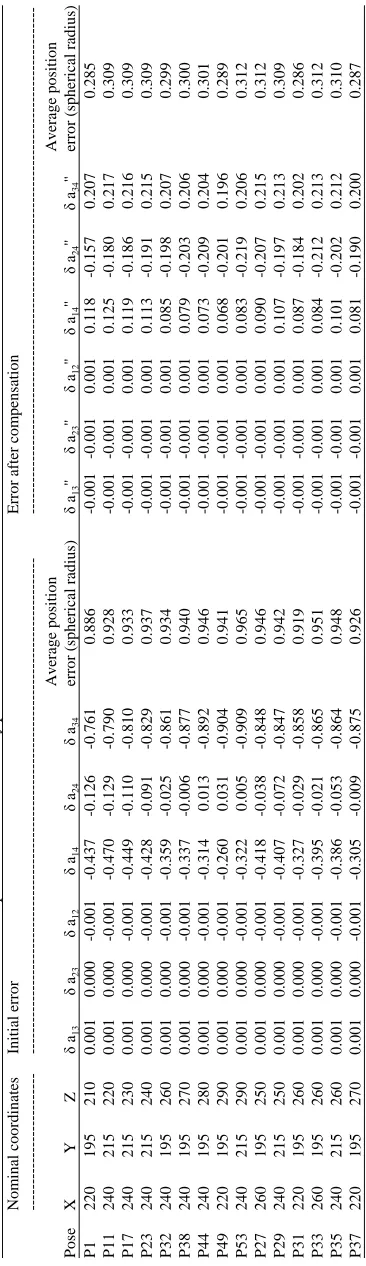
[image:7.612.73.543.516.727.2]Compensation of end-effector error based on interpolation results: Using the compensatory solutions proposed in section 3, the research team conducted a survey at 15 random poses in the prism. The calculation position for compensation was taken from a comparison between two values: the position after being predicted by the shape function and the nominal one. The inverse kinematic problem is then solved to acquire the set of joint variables for the actual control process. Data collected with the ABB robot before and after compensation is summarized in Table 5.
Table 4: Verifying end-effector errors at certain poses
Nominal coordinates End-effector errors from direct measurements End-effector errors from interpolating shape function --- --- ---Pose X Y Z δ a13 δ a23 δ a12 δ a14 δa24 δ a34 δ a13 δ a23 δ a12 δ a14 δa24 δ a34
T
able 5: Robot
end-effector er ro rs befor e and after com p
ensation at r
[image:8.612.220.403.96.729.2]0 2 4 6 8 10 12 14 16 18 20 Point
-0.26
-0.28
-0.30
-0.32
-0.34
-0.36
-0.38
-0.40
-0.42
-0.44
-0.46
P
o
siti
o
n
e
rr
o
r i
n
x-d
ir
ecti
o
n
(
m
m
)
Errors in X-direction
Directly measured error Predicted error (a)
0 2 4 6 8 10 12 14 16 18 20 Point
0.18
0.16
0.14
0.12
0.10
0.08
0.06
0.04
0.02
P
o
sitio
n er
ro
r i
n
y
-d
ir
ection
(
m
m
)
Errors in Y-direction (b)
0 2 4 6 8 10 12 14 16 18 20 Point
0.40
0.39
0.38
0.37
0.36
0.35
0.34
0.33
0.32
0.32
0.31
P
o
si
tio
n
e
rr
o
r in
z-dir
ec
tio
n
(
m
m
)
Errors in Z-direction (c)
0 1 2 3 4 5 6 7 8 9 10 11 12 13 14 15 Point
1.0
0.9 0.8
0.7 0.6
0.5 0.4
0.3 0.2
0.0
XY
Z
e
rr
o
r
(m
m
)
+ + + + + + + + + + + + + + + +
Errors without calibration Errors with calibration
[image:9.612.95.521.86.459.2]Fig. 8(a-c): Position errors of the end-effector measured experimentally and determined by the shape function in the X, Y and Z directions
Fig. 9: Comparison of end-effector errors before (red) and after (blue) calibration
The graph in Fig. 9 shows the position error values of the robotin the workspace before and after compensation. In the figure, the red line represents the errors without calibration andthe blue represents those with calibration.
With the calibration of the joint variable, the end-effector position accuracy was significantly improved (the average error decreased from 0.936-0.302 mm). This demonstrates the correctness and efficiency of the proposed method.
CONCLUSION
[image:9.612.81.294.495.634.2]not affect the robot, nor require a significant amount of time to implement. The method can also be applied to many different types of robots, regardless of the number of DOF or type of workspace.
ACKNOWLEDGEMENTS
This research was supported by the Thai Nguyen University of Technology (TNUT) of Vietnam (T2019-B07 project).
REFERENCES
Abderrahim, M., A. Khamis, S. Garrido, L. Moreno and L.K. Huat, 2006. Accuracy and Calibration Issues of Industrial Manipulators. In: Industrial Robotics: Programming, Simulation and Applications, Huat, L.K. (Ed.). IntechOpen, London, UK., ISBN:3-86611-286-6, pp: 131-135.
Bai, Y. and D. Wang, 2003a. Improve the position measurement accuracy using a dynamic on-line fuzzy interpolation technique. Proceedings of the 3rd International Workshop on Scientific use of Submarine Cables and Related Technologies, July 31-31, 2003, IEEE, Lugano, Switzerland, pp: 227-232.
Bai, Y. and D. Wang, 2003b. On the comparison of interpolation techniques for robotic position compensation. Proceedings of the Joint 2003 IEEE International Conference on Systems, Man and Cybernetics SMC'03 and Theme-System Security and Assurance (Cat. No.03CH37483) Vol. 4, October 8, 2003, IEEE, Washington, DC., USA., pp: 3384-3389.
Bai, Y. and D. Wang, 2004. Improve the robot calibration accuracy using a dynamic online fuzzy error mapping system. IEEE. Trans. Syst. Man Cybern. Part B., 34: 1155-1160.
Bai, Y. and D. Wang, 2006. Fuzzy Logic for Robots Calibration-Using Fuzzy Interpolation Technique in Modeless Robot Calibration. In: Advanced Fuzzy Logic Technologies in Industrial Applications, Bai, Y., H. Zhuang and D. Wang (Eds.). Springer, London, UK., ISBN:978-1-84628-468-7, pp: 299-313.
Bai, Y. and D. Wang, 2016. On the comparison of an interval Type-2 Fuzzy interpolation system and other interpolation methods used in industrial modeless robotic calibrations. Proceedings of the 2016 IEEE International Conference on Computational Intelligence and Virtual Environments for Measurement Systems and Applications (CIVEMSA), June 27-28, 2016, IEEE, Budapest, Hungary, ISBN:978-1-4673-9760-5, pp: 1-6.
Bai, Y. and H. Zhuang, 2004. On the comparison of model-based and modeless robotic calibration based on the fuzzy interpolation Technique. Proceedings of the International IEEE Conference on Robotics, Automation and Mechatronics, December 1-3, 2004, IEEE, Singapore, pp: 892-897.
Bai, Y. and H. Zhuang, 2005. On the comparison of bilinear, cubic spline and fuzzy interpolation techniques for robotic position measurements. IEEE. Trans. Instrum. Meas., 54: 2281-2288.
Bai, Y., J.C. Smith, H. Zhuang and D. Wang, 2008. Calibration of parallel machine tools using fuzzy interpolation method. Proceedings of the 2008 IEEE International Conference on Technologies for Practical Robot Applications, November 10-11, 2008, IEEE, Woburn, Massachusetts, USA., ISBN:978-1-4244-2791-8, pp: 56-61.
Borrmann, C. and J. Wollnack, 2014. Calibration of external linear robot axes using spline interpolation. Proceedings of the 2014 International Conference on Modelling, Identification & Control, December 3-5, 2014, IEEE, Melbourne, Australia, pp: 111-116.
Conrad, K.L., P.S. Shiakolas and T.C. Yih, 2000. Robotic calibration issues: Accuracy, repeatability and calibration. Proceedings of the 8th Mediterranean Conference on Control and Automation (MED2000), July 17-19, 2000, Rio, Patras, Greece, pp: 1-6. Hayati, S., K. Tso and G. Roston, 1988. Robot geometry
calibration. Proceedings of the 1988 IEEE International Conference on Robotics and Automation, April 24-29, 1988, IEEE, Philadelphia, Pennsylvania, USA., pp: 947-951.
Kamali, K., A. Joubair, I.A. Bonev and P. Bigras, 2016. Elasto-geometrical calibration of an industrial robot under multidirectional external loads using a laser tracker. Proceedings of the 2016 IEEE International Conference on Robotics and Automation (ICRA), May 16-21, 2016, IEEE, Stockholm, Sweden, pp: 4320-4327.
Kong, L., G. Chen, Z. Zhang and H. Wang, 2018. Kinematic calibration and investigation of the influence of universal joint errors on accuracy improvement for a 3-DOF parallel manipulator. Rob. Comput. Integr. Manuf., 49: 388-397.
Liu, Z., J. Xu, Q. Cheng, Y. Zhao, Y. Pei and C. Yang, 2018. Trajectory planning with minimum synthesis error for industrial robots using screw theory. Intl. J. Precis. Eng. Manuf., 19: 183-193.
Mooring, B.W., Z.S. Roth and M.R. Driels, 1991. Fundamentals of Manipulator Calibration. Wiley, New York, USA., ISBN:9780471508649, Pages: 329.
Sun, T., Y. Zhai, Y. Song and J. Zhang, 2016. Kinematic calibration of a 3-DoF rotational parallel manipulator using laser tracker. Rob. Comput. Integr. Manuf., 41: 78-91.
Wang, D., Y. Bai and J. Zhao, 2012. Robot manipulator calibration using neural network and a camera-based measurement system. Trans. Inst. Meas. Control, 34: 105-121.
Wang, S.M., Y.L. Liu and Y. Kang, 2002. An efficient error compensation system for CNC multi-axis machines. Intl. J. Mach. Tools Manuf., 42: 1235-1245.
Weill, R. and B. Shani, 1991. Assessment of accuracy of robots in relation with geometrical tolerances in robot links. CIRP. Annals, 40: 395-399.