On the stress update algorithm of an advanced critical state elasto plastic model and the effect of yield function equation

http://wrap.warwick.ac.uk

Original citation:

Rezania, Mohammad, Sivasithamparam, Nallathamby and Mousavi Nezhad,

Mohaddeseh. (2014) On the stress update algorithm of an advanced critical state

elasto-plastic model and the effect of yield function equation. Finite Elements in Analysis and

Design, Volume 90 . pp. 74-83. ISSN 0168-874X

Permanent WRAP url:

http://wrap.warwick.ac.uk/62058

Copyright and reuse:

The Warwick Research Archive Portal (WRAP) makes this work of researchers of the

University of Warwick available open access under the following conditions.

This article is made available under the Creative Commons Attribution 3.0 (CC BY 3.0)

license and may be reused according to the conditions of the license. For more details

see:

http://creativecommons.org/licenses/by/3.0/

A note on versions:

The version presented in WRAP is the published version, or, version of record, and may

be cited as it appears here.

On the stress update algorithm of an advanced critical state

elasto-plastic model and the effect of yield function equation

Mohammad Rezania

a,n

, Nallathamby Sivasithamparam

b

, Mohaddeseh Mousavi Nezhad

c

a

Nottingham Centre for Geomechanics, Department of Civil Engineering, Faculty of Engineering, University of Nottingham, Nottingham NG7 2RD, UK

b_{Offshore Energy, Computational Geomechanics (CGM), Norwegian Geotechnical Institute, NO-0806 Oslo, Norway} c

Computational Mechanics, Civil Research Group, School of Engineering, University of Warwick, Warwick CV4 7AL, UK

a r t i c l e i n f o

Article history:

Received 21 November 2013 Received in revised form 14 May 2014

Accepted 18 June 2014

Keywords:

Constitutive modelling Elasto-plasticity Stress integration Numerical simulation

a b s t r a c t

This paper investigates the computational performance of S-CLAY1S constitutive model by varying its yield function equation. S-CLAY1S is an advanced anisotropic elasto-plastic model that has been developed based on the extension of conventional critical state theory. In addition to modified Cam-Clay's hardening law, S-CLAY1S also accounts for inherent and evolving plastic anisotropy, interparticle bonding and degradation of bonds during plastic straining. A modified Newton–Raphson stress update algorithm has been adopted for the implementation of the model and it was found that the algorithm's convergence performance is sensitive to the expression of the yield function. It is shown that for an elasto-plastic model which is developed based on the critical state theory, it is possible to improve the performance of the numerical implementation by changing the form of the yield function. The results of this work can provide a new perspective for computationally cost-effective implementation of complex constitutive models infinite element analysis that can yield in more efficient boundary value level simulations.

&2014 The Authors. Published by Elsevier B.V. This is an open access article under the CC BY license (http://creativecommons.org/licenses/by/3.0/).

1. Introduction

It is a well-established fact in soil mechanics that the yield curves obtained from experimental tests (with triaxial or hollow cylinder apparatuses) on undisturbed samples of natural clays are inclined due to the inherent fabric anisotropy in the soil's structure (e.g. [1_–3]). Since consideration of full anisotropy in modelling soil's behaviour is not practical due to the number of parameters involved, efforts have been mainly focused on the development of models with reduced number of parameters while maintaining the capacity of the model [4]. In order to capture the effects of anisotropy on soil's behaviour, a number of researcher have proposed anisotropic elasto-plastic constitutive models involving an inclined yield curve that is eitherfixed (e.g.[5]) or is able to rotate in order to simulate the development or erasure of aniso-tropy during plastic straining (e.g.[6–9]). Among the developed anisotropic models, S-CLAY1S model[10]has been well-validated and accepted as a practical anisotropic model for simulating natural clays' behaviour (e.g.[11–13]). The consideration of aniso-tropy in this model is similar to an earlier version of the model called S-CLAY1 [8]. In both S-CLAY1 and S-CLAY1S models the

initial anisotropy is assumed to be cross-anisotropic, which is a realistic assumption for normally consolidated clays deposited along the direction of consolidation. Both models account for the development or erasure of anisotropy if the subsequent loading produces irrecoverable strains, resulting a generalised plastic anisotropy condition. S-CLAY1S model is further extended to account for inter-particle bonding in natural soil's structure, and subsequent destructuration of bonds when the soil is under plastic straining. The main advantages of S-CLAY1S model over other proposed anisotropic models are (i) its realisticK0prediction, and

most importantly (ii) the fact that model parameter values can be determined from standard laboratory tests using well-defined methodologies[10].

With additional complexity of a constitutive model, comes additional computational cost for its application. Particularly implementation of advanced constitutive models to solve bound-ary value problems requires integration algorithms that are not only stable, robust and accurate but also computationally efficient; because, in this case, the number of calculations involved per analysis increment is much higher than in the case of simple element level simulations for model validation. The main problem for successful implementation of complex constitutive models in thefinite element method is error control that is the result of adoptingfinite number of loading steps. There are generally two techniques to solve a constitutive model's system of equations at a stress point, the explicit (incremental) method and the implicit Contents lists available atScienceDirect

journal homepage:www.elsevier.com/locate/finel

Finite Elements in Analysis and Design

http://dx.doi.org/10.1016/j.finel.2014.06.009

0168-874X/&2014 The Authors. Published by Elsevier B.V. This is an open access article under the CC BY license (http://creativecommons.org/licenses/by/3.0/). n_{Corresponding author. Tel.:þ44 115 951 3889.}

E-mail addresses:[email protected](M. Rezania), [email protected](N. Sivasithamparam),

[email protected](M. Mousavi Nezhad).

(iterative) method. In the explicit method the solution is approached using the previously known stress point's response in order to approximate the nonlinear material behaviour. This method is popular within the research community mainly due to its simplicity. However, the main issue in an explicit algorithm is that its success largely relies on the size of the incremental load steps, therefore the results particularly at boundary value level, can be load step dependant. This problem usually results in limiting the application of an advanced constitutive model at practical level. Nevertheless, there are modifications such as adopting an automatic substepping technique [14] to improve the performance of an explicit implementation. In the implicit or so-called return mapping algorithm[15]the constitutive model's governing equations are treated nonlinearly and are solved in an iterative manner until the drift from the yield surface is small enough[16]. In this method the computed stress state automati-cally satisfies the yield condition. Also it does not need the computation of the intersection with the yield surface as the stress state changes from elastic to elasto-plastic[17]. The implicit method is particularly attractive if the model is to be used for practical simulations, which is mainly due to the fact that it is much more stable and efficient. However its application for advanced constitutive models is very difficult as it requires second order derivatives of the yield function.

In this study the return mapping algorithm [15] has been utilised for integrating the S-CLAY1S model. Previously, the appli-cations of the return mapping algorithm to the modified Cam-Clay (MCC) model[18], through implicit and semi-implicit integration schemes, were investigated in [16,17]. It was found that the algorithm is capable of efficiently solving the nonlinear system of equations of the MCC model even during large strain incre-ments. More recently Pipatpongsa et al. have shown that the form of the MCC's yield function influences the performance of their developed backward Euler stress update algorithm for the model [19]; and, in case of original Cam-Clay model [20] the success or failure of their semi-implicit implementation has also been dependant on the yield function's form [21]. In a separate work, Coombs and Crouch[22]have demonstrated the effects that alternative expressions of yield function has on the robustness and efficiency of a backward Euler stress integration method for a critical state based hyperplastic model.

In this paper a new Modified Newton–Raphson stress update scheme is employed for the numerical implementation of the

S-CLAY1S model. The scheme has proven to have very high efficiency, robustness and accuracy for integrating the constitutive relationship during incremental elasto-plastic response[23]. It is also shown that the yield function form of the S-CLAY1S model can be presented with different alternative formulations; therefore, the corresponding solution algorithm results in different conver-gence speeds depending on which form of the yield function is used. Through model performance comparisons the most suitable formulation of the advanced anisotropic model is identified for its implementation.

2. S-CLAY1S model

The S-CLAY1S is an advanced critical state model which accounts for bonding and destructuration, in addition to plastic anisotropy[10]. In three-dimensional stress space the yield surface of the S-CLAY1S model, fy, is a sheared ellipsoid (seeFig. 1(a))

defined as

fy¼

3 2½f

σ

dp

0

_α

dgTf

σ

dp0

α

dg M2

3 2f

α

dg

T_f

_α

dg

ðp0mp0Þp0¼0

ð1Þ

In the above equation

σ

dand

α

dare the deviatoric stress tensor

and the deviatoric fabric tensor respectively,Mis the critical state value,p0is the mean effective stress, andp0mis the size of the yield

surface related to the soil's preconsolidation pressure. The effect of bonding in the S-CLAY1S model is described by an intrinsic yield surface [24] which has the same shape and inclination of the natural yield surface but with a smaller size. The size of the intrinsic yield surface is specified by parameterp0

mithat is related

to the sizep0m of the natural yield surface by parameter

χ

as the

current amount of bonding

p0m¼ ð1þ

χ

Þp0mi ð2Þ

S-CLAY1S model incorporates three hardening laws. Thefirst of these, relates the increase in the size of the intrinsic yield surface to the increments of plastic volumetric strain (d

ε

pv)

dp0mi¼

vp0

mi

λ

i

κ

d

ε

p

v ð3Þ

where

ν

is the specific volume,

λ

i is the gradient of the intrinsic

normal compression line in the compression plane (lnp0

_ν

Nomenclature

α

0,

α

initial and current value of anisotropy

α

d deviatoric fabric tensor

d

α

change in scalar value of anisotropy d

ε

pv incremental volumetric plastic strain

d

ε

p_d incremental deviatoric plastic strain d

χ

change in value of bonding

½De elastic constitutive matrix

ε

e_,

ε

p _{elastic and plastic strain vector}

ε

e;tr _{trial elastic strain vector}

fy,f e

y yield function and trial value of yield function

G0 shear modulus H1,H2,H3 hardening moduli

η

stress ratio

K0 lateral earth pressure at rest

κ

swelling index

λ

compression index

λ

i intrinsic compression index

Λ

plastic multiplier

M stress ratio at critical state

ν

specific volume

ξ

rate of destructuration

ξ

d rate of destructuration due to deviator stress

OCR over-consolidation ratio p0 mean effective stress

p0m effective preconsolidation pressure

p0_mi size of intrinsic yield curve q deviatoric stress

r_ε,rf residual errors

RTOL,FTOL tolerance values

σ

0 _{effective stress state}

σ

0

d deviatoric effective stress vector

υ

0 _{poisson's ratio}

χ0

,

χ

initial and current value of bonding

ω

rate of rotation

space), and

κ

is the slope of the swelling line in the compression plane. The second hardening law is the rotational hardening law, which describes the rotation of the yield surface with plastic straining[8]

d

α

d¼

ω

3

η

4

α

d

〈d

ε

p v〉þ

ω

d

η

3

α

d

h i

d

ε

p_d

ð4Þ

where

η

is the tensorial equivalent of the stress ratio defined as

η

¼

_σ

d=p0,d

ε

pdis the increment of plastic deviatoric strain, and

ω

and

ω

dare additional soil constants that control, respectively, the absolute rate of the rotation of the yield surface toward its current target value, and the relative effectiveness of plastic deviatoric strains and plastic volumetric strains in rotating the yield surface. The third hardening law in S-CLAY1S is destructuration, which describes the degradation of bonding with plastic straining. The destructuration law is formulated in such a way that both plastic volumetric strains and plastic shear strains tend to decrease the value of the bonding parameter

χ

towards a target value of zero[10], it is defined as

d

χ

¼

_ξχ

ðjd

ε

p

vjþ

ξ

djd

ε

p

djÞ ð5Þ

where

ξ

and

ξ

dare additional soil constants. Parameter

ξ

controls the absolute rate of destructuration, and parameter

ξ

dcontrols the relative effectiveness of plastic deviatoric strains and plastic volumetric strains in destroying the inter-particle bonding[25].

[image:4.595.117.467.57.215.2]

The elastic behaviour in the model is formulated with the same isotropic relationship as in MCC model[18]requiring the values of two parameters;

κ

and the Poisson's ratio,

ν

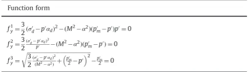
0(to evaluate the value of elastic shear modulus G0). By mathematical manipulation of Eq. (1)different forms of the yield function can be defined for the S-CLAY1S model, from which three different forms are summarised in

Table 1. From the yield function forms listed inTable 1,f1yis the

original S-CLAY1S yield function expressed in the triaxial stress space, and the other two forms are additional alternatives for the model which are also presented in the triaxial stress space.

3. S-CLAY1S implementation

The Modified Newton–Raphson (MNR) integration scheme involves iterative procedure to solve nonlinear system of strain-driven formulation. Two sets of residual equations are formulated and solved by the MNR method. The first set of equations is constitutive relations in terms of strain components and the second set is a constraint equation in terms of yield function. In what follows the standard notation is adopted in which the elastic and plastic parts of strain,

ε

, are denoted by superscriptse and p respectively. In the basics of elasto-plastic theory it is assumed that the total strain increment consists of elastic strain

increment and plastic strain increment as

Δε

¼

_Δε

e_þ

_Δε

p _ð6Þ

where

Δ

remarks an incremental operator, and the underlined strain symbolises its vector form. Assuming an associatedflow rule for evaluating plastic strain increments,

Δε

p_{, we have}

Δε

¼

_Δε

e_þ

_ΔΛ

∂fy

∂

σ

0 ð7aÞ

hence the stress increment for a given trial strain can be obtained from

Δσ

0_{¼ ½}

De

_Δε

½De

_ΔΛ

∂fy

∂

σ

0 ð7bÞ

where

Λ

is the so-called plastic multiplier,

σ

0is the effective stress and ½De is the elastic constitutive matrix. To derive the plastic multiplier of the S-CLAY1S model, the yield function can be expanded with the Taylor series expansion approach [23], by ignoring second or higher order terms we have

fy¼f

e yþ

∂fy

∂

σ

0

Δσ

0þ ∂fy

∂p0

mi

Δ

p0miþ

∂fy

∂

α

Δα

þ ∂fy

∂

χ

Δχ

ð7cÞ

whenfeyis the so-called trial yield function value. Given that the

strain increment has all been applied to arrive at the elastic stress predictor, the MNR algorithm involves zero strain increment. Therefore Eq.(7-b)becomes

Δσ

0_{¼ ½D}e

_ΔΛ

∂fy

∂

σ

0 ð7dÞ

The yield function value in Eq. (7-c)is zero as a stress state cannot stay outside the yield surface, therefore by using Eqs.(7-c)

Table 1

Alternative forms for the S-CLAY1S yield function,fy.

Function form

f1y¼ 3

2ðσ0dp0αdÞ2ðM2α2Þðp0mp0Þp0¼0

f2

y¼ 3 2 ðσ0

dp 0_α

dÞ2

p0 ðM2α2Þðp0mp0Þ ¼0

f3y¼

ffiffiffiffiffiffiffiffiffiffiffiffiffiffiffiffiffiffiffiffiffiffiffiffiffiffiffiffiffiffiffiffiffiffiffiffiffiffiffiffiffiffiffiffiffiffiffi

3 2 ðσ0

dp 0_α

dÞ2 ðM2_α2Þþ

p0 m

2p0

2

r

p0 m

2¼0

whereσdis the deviatoric stress tensor;p0is the mean effective stress;αdis the deviatoric fabric tensor;α is a scalar parameter for the special case of

cross-anisotropy and its value is obtained asα¼ ffiffiffiffiffiffiffiffiffiffiffiffiffiffiffiffiffiffiffiffiffiffiffiffiffiffiffiffiffiffiffið3=2ÞfαdgTfαdg

q

;Mis the value of the stress ratio at critical state; andp0

mis the size of the yield surface. Intrinsic yield surface

q

p

′

M 1

1 α

pm pmi

Natural yield surface

[image:4.595.300.554.260.334.2]

′ ′

Fig. 1.S-CLAY1S yield surface represented in (a) three dimensional stress space, and (b) triaxial stress space.

M. Rezania et al. / Finite Elements in Analysis and Design 90 (2014) 74–83

and (7-d), the plastic multiplier is derived as

ΔΛ

¼ f

e y

½∂fy=∂

σ

0Tð½DeU½∂fy=∂

σ

0Þþ

Η

1þ

Η

2þ

Η

3

ð8aÞ

where

Η

1¼∂ fy

∂p0_miU

∂p0_mi

∂

ε

p vU

∂fy

∂p0 ð8bÞ

Η

2¼ ∂

fy

∂

α

d

( )T

U ∂

α

d

∂

ε

p v

U ∂fy

∂p0

þ ∂

α

d

∂

ε

p d ( ) U ffiffiffiffiffiffiffiffiffiffiffiffiffiffiffiffiffiffiffiffiffiffiffiffiffiffiffiffiffiffiffiffiffiffiffiffiffiffiffiffiffiffiffi 2 3U

∂fy

∂

σ

0

d

( )T

U ∂fy

∂

σ

0

d ( ) v u u t 2 6 4 3 7 5

ð8cÞ

Η

3¼∂ fy

∂

χ

U ∂∂

ε

χ

p vU

∂fy

∂p0

þ∂x

∂

ε

p d

U

ffiffiffiffiffiffiffiffiffiffiffiffiffiffiffiffiffiffiffiffiffiffiffiffiffiffiffiffiffiffiffiffiffiffiffiffiffiffiffiffiffiffiffi

2 3U

∂fy

∂

σ

0

d

( )T

U ∂fy

∂

σ

0

d ( ) v u u t 2 6 4 3 7

5 ð8dÞ

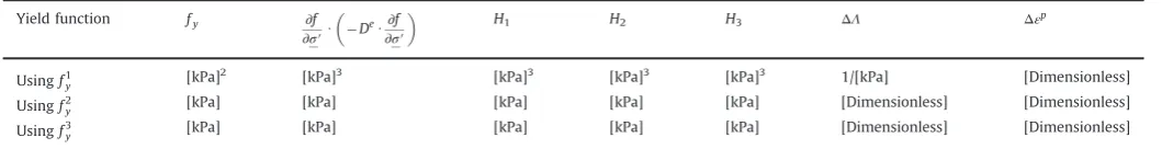
[image:5.595.41.571.80.148.2] [image:5.595.44.296.569.710.2]

Dimensional analysis of Eq. (7-a) is required to determine whether it is correct to use any of the three yield function forms, presented inTable 1, in the MNR algorithm. Thefirst two terms of the Eq.(7-a)are strains and therefore dimensionless, hence the third term, i.e. the plastic strain increment, must also be dimen-sionless. The results of the dimensional analysis are summarised in

Table 2with SI units used in the analyses.

As it is seen in the table, all three yield functions result in dimensionless plastic strain increment, therefore they are all dimen-sionally consistent and suitable to be used in the MNR process. The two sets of residual equations in the developed MNR algorithm are

r_ε¼

_Δε

_Δε

e;tr

_ΔΛ

∂fy

∂

σ

0 ð9aÞ

and

rf¼fyð

σ

0Þ ð9bÞ

Differentiating the residuals in equations above with regards to the stresses leads a set of linearised equations which, after neglecting higher order terms, can be written in an iterative manner as follows

Δε

n

Δε

e n

δΔε

e

nþ1

ΔΛ

n ∂fy

∂

σ

0

n

_ΔΛ

n ∂

2_f

y

∂

σ

0

nþ1

2δσ0

nþ1

ΔΛ

nþ1∂ fy

∂

σ

0

n

¼0

ð10aÞ

fyþ

∂fy

∂

σ

0

n

δσ

0

nþ1¼0 ð10bÞ

Eq.(10)can be expressed in the matrix form as

Iþ

ΔΛ

n ∂

2_f y

∂σ0

nþ1

2½D

e nþ1 ∂

fy

∂σ0

n

∂fy

∂σ0

nD

e

nþ1 0

2 6 4 3 7 5

δΔε

e nþ1

δΔΛ

nþ1

8 > < > : 9 > = > ;¼ r_ε rf 8 > > > > > < > > > > > : 9 > > > > > = > > > > > ;

ð11Þ

whereIis the fourth order identity tensor. The above system of equations is solved in an iterative manner, and as the result the changes of elastic strain increment and the plastic multiplier will

be obtained. The state variables of the model are updated in every iteration, and the procedure of updating

Δε

and

ΔΛ

within a load step is repeated until the norms of both residuals, i.e.rεandrfare

less than the prescribed tolerances, namely RTOL and FTOL. Now the trial elastic strain increment,

Δε

e;tr_{, is defined by the}

following equation where

Δε

e

i is the initial elastic strain increment

converged in the previous step and

δΔε

e _{is the changes of}

elastic strain increment obtained from the above system of equations

Δε

e;tr_¼

_Δε

e iþ

δΔε

e _ð12Þ

Accordingly the trial value of plastic multiplier gets updated too. The yield function,fy, appears in Eq.(11)can be replaced by

individual yield functions listed inTable 1.

4. Computational performance

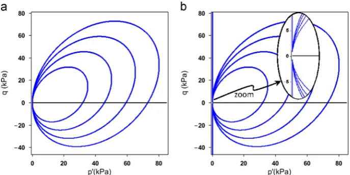
Different formulations of the S-CLAY1S yield function are all representing similar equation when equating to zero, therefore they are supposed to produce unique surfaces. However, in the triaxial stress spacef2yresults in numerical singularity when mean

effective stress (i.e.p0) closes to zero (seeFig. 2) which simply is due to the presence of p0 in the denominator term of the equation (seeTable 1).

It is commonly known that critical state models do not have any strength if the effective mean stress is zero or tensile, there-fore for them to be successfully used a compressive initial stress state is required to be established at the point of interest in the numerical domain. Taking this into account, there is not a particular dif_ficulty in consideringf2_yin the model implementation and its application. In the following, assessments of the proposed MNR numerical algorithm for S-CLAY1S integration with regards to each alternative form of the yield function will be presented. Because the S-CLAY1S model is already validated (e.g.,[11–13]), in this paper only the numerical performance of the proposed algorithm is studied, and the effect of the yield function equation on the proposed stress update scheme is investigated.

4.1. At stress point level

A set of parameter values for the S-CLAY1S constitutive model representing a well-known soft clay, namely Bothkennar clay, is selected in order to demonstrate the computational performance of the model implementation (seeTable 3). Bothkennar clay is a soft normally consolidated marine clay deposited on the Forth River Estuary which is located approximately midway between Glasgow and Edinburgh in Scotland. There is extensive laboratory data available for Bothkennar clay (e.g., [26]) which makes it possible to derive a consistent set of material parameters for the advanced constitutive model being studied. The details of para-meter determination can be found in[26,27].

At first stage, the verification of the implementation is per-formed by using an in-house developed integration point pro-gramme (IPP). The S-CLAY1S model subroutine is strain driven, i.e. known increments in strain are input to the model and the Table 2

Results of dimensional analyses forΔεp

using different yield function forms.

Yield function fy ∂f ∂σ0U DeU

∂f

∂σ0

H1 H2 H3 ΔΛ Δεp

Usingf1y [kPa]

2 _[kPa]3 _[kPa]3 _[kPa]3 _[kPa]3 _{1/[kPa] [Dimensionless]}

Usingf2

y [kPa] [kPa] [kPa] [kPa] [kPa] [Dimensionless] [Dimensionless] Usingf3

corresponding stresses are output. Thus, by specifying strain increments and the material parameters, the corresponding stress output can be used for evaluating model performance without the need for any finite element (FE) software. Depending on which form of the yield function is employed in the implementation, the convergence speed of the iterative scheme would vary as it depends on the degree of nonlinearity in the system of governing equations.

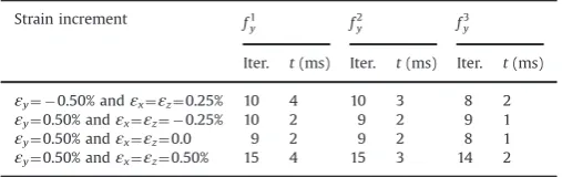
Different combinations of strain loading have been considered in the way that they cover many important stress–strain condi-tions in common soil element tests. In each case an identical initial stress inside the yield surface was selected and then under a specific loading condition the stress path was monitored. The magnitudes of the imposed strains were selected in the way that they cover a significant range of loading conditions. A summary of the applied strains are shown in thefirst column ofTable 4. The performance of the implementation using different functions can be studied by analysing their efficiency which can be represented by the number of iterations required for convergence. As it is seen inTable 4, for the majority of loading cases, the employment off3y

results in the lowest number of iterations. Yield function equations

f1y and f

2

y generally seem to produce very similar number of

iterations. Table 4 also shows the required CPU time (in milli-seconds) for each analysis. The measured computational times for the analyses are based on a PC with an Intel Core i7-3820 3.60 GHz processor, and they are recorded using the standard SYSTEM_ CLOCK subroutine [28] in Lahey/Fujitsu FORTRAN Professional V7.3 compiler. Even though in real-time scale the durations of analyses are almost indifferent; however, in computational sense f3yis evidently cheaper as compared to the other two forms of the

yield function, its application results in solutions being converged within less CPU time.

Stress return paths for cases representing more commonly observed conditions in soil tests are presented in Fig. 3. Among them, Fig. 3(a)–(c) represents triaxial undrained compression, undrained extension and isotropic compression conditions respec-tively, andFig. 3(d) represents oedometer condition (one dimen-sional straining).

It is seen that in all cases of different given strain increments, the return mappings of the arbitrary trial stresses converge to identicalfinal stresses on the yield surface; that is an indication of the robustness of developed MNR algorithm. However, the return mapping paths and the required number of iterations vary depending on the form of the yield function. This is mainly because the direction of stress return path depends on different derivations of the yield function (with regards to stresses and/or state variables, assuming associatedflow rule) which are dissim-ilar when different yield function equations are employed. From the results, it is noteworthy to mention that in thefirst iterationf2_y employment usually produces the most erroneous stress value compared to when the other two forms are used (seeFigs. 3(a), (c) and (d)).

In order to obtain more insight into the possible sensitivity of the MNR algorithm to the variations of the yield surface shape, a simple sensitivity analysis is likely to be helpful. Based on the authors' experience the S-CLAY1S model performance is not particularly sensitive to different, but yet appropriate, combina-tions of constant values in rotational and destructuration hard-ening laws, namely

ω

,

ω

d,

ξ

and

ξ

d. Therefore, for the sake of simplicity, the sensitivity analysis has only been performed within an upper and lower plausible limit for state variables

α

0and

χ

0.

Four different series of analyses have been done with changing each of

α

0 and

χ

0 values by 725% around their representative

values listed inTable 3. Only the four stress paths illustrated in

[image:6.595.121.465.57.229.2]

Fig. 3are simulated and the results of the analyses are summarised inTables 5–8. Looking at the results in these tables and comparing Table 3

Material parameters for S-CLAY1S representing Bothkennar clay.

[image:6.595.31.285.292.325.2]

e0 OCR α0 χ0 κ υ λi M ω ωd ξ ξd 2.0 1.5 0.59 8.0 0.02 0.2 0.18 1.5 50 1.0 9 0.2

Table 4

Imposed strain increments for single stress level analyses of S-CLAY1S model, the required number of iterations for convergence, and the required CPU time for the analysis (in milliseconds) depending on the yield function form.

Strain increment f1

y f2y f3y

Iter. t(ms) Iter. t(ms) Iter. t(ms)

εy¼ 0.50% andεx¼εz¼0.25% 10 4 10 3 8 2

εy¼0.50% andεx¼εz¼ 0.25% 10 2 10 2 9 1

εy¼0.50% andεx¼εz¼0.0 9 2 9 2 8 1

εy¼0.50% andεx¼εz¼0.25% 12 3 11 2 11 2

εy¼0.50% andεx¼εz¼0.05% 10 2 10 2 8 1

εy¼0.50% andεx¼εz¼0.10% 10 2 10 2 8 1

εy¼0.50% andεx¼εz¼0.20% 11 3 10 2 10 1

εy¼0.50% andεx¼εz¼0.30% 13 3 11 2 12 2

εy¼0.50% andεx¼εz¼0.40% 14 3 14 2 13 2

εy¼0.50% andεx¼εz¼0.50% 15 4 15 3 14 2 Fig. 2.Contours of arbitrary S-CLAY1S yield surfaces in triaxial stress space using (a)f1yorf

3

y, and (b)f

2

y.

M. Rezania et al. / Finite Elements in Analysis and Design 90 (2014) 74–83

[image:6.595.305.551.309.441.2]

them with those summarised inTable 4, it can be seen that there is not a dramatic change in how the MNR algorithm performs using different yield function forms. It is observed that the employment off3_y in the stress return algorithm continues to outperform the performance of the algorithm when the other two forms of the yield function are used. The number of iterations and CPU times are mostly identical or close to the corresponding ones inTable 5

which would be expected given that the imposed single-step loadings are the same and in each case only the shape of the yield surface is tweaked to some extent.

4.2. At boundary value level

To compare the numerical performance of the implicit integra-tion scheme described in the previous secintegra-tion at boundary value level, a relatively simple example is analysed withfinite element method. The boundary value problem involves plane strain ana-lysis of a hypothetical embankment constructed on a soft soil deposit with the properties of Bothkennar clay. This is a good case for assessing the performance of the integration algorithm with different yield function forms due to the significant rotation of principal stresses [29] particularly in areas directly below the embankment. The S-CLAY1S model has been implemented into PLAXISfinite element programme as a user-defined soil model in

50 100 150 200

50 75 100

q (kPa)

p' (kPa)

f ; 10 iterations f ; 10 iterations f ; 8 iterations Initial yield surface Final yield surface σ′tri

σ′int σ′f

εx= 0.25%

εy= -0.50%

εz= 0.25%

-75 -50 -25 0 25 50

50 75 100

q (kPa)

p' (kPa)

f ; 10 iterations f ; 10 iterations f ; 9 iterations Initial yield surface Final yield surface σ′_tri

σ′int

σ′_f

εx= -0.25%

εy= 0.50%

εz= -0.25%

50 75 100 125 150

q (kPa)

p' (kPa) f ; 9 iterations f ; 9 iterations f ; 8 iterations Initial yield surface Final yield surface

σ′int σ′f

σ′tri

εx= 0.0

εy= 0.50%

εz= 0.0

25 50 75 100

50 75 100 125 50 100 150 200 250

q (kPa)

p' (kPa)

f ; 15 iterations f ; 15 iterations f ; 14 iterations Initial yield surface Final yield surface

σ′tri

σ′_f σ′int

εx= 0.50%

εy= 0.50%

[image:7.595.129.477.57.318.2]

εz= 0.50%

[image:7.595.309.562.394.474.2]

Fig. 3.Return-mapping paths for four different sets of imposed strain increments.

Table 5

Sensitivity of the Newton–Raphson stress update scheme to the variations of the yield surface shape by a 25% increase in theα0value.

Strain increment _f1

y f

2

y f

3

y

Iter. t(ms) Iter. t(ms) Iter. t(ms)

εy¼ 0.50% andεx¼εz¼0.25% 10 4 10 3 8 2

εy¼0.50% andεx¼εz¼ 0.25% 9 2 9 2 9 1

εy¼0.50% andεx¼εz¼0.0 10 2 9 2 8 1

[image:7.595.40.291.395.474.2]

εy¼0.50% andεx¼εz¼0.50% 15 4 16 3 15 2

Table 6

Sensitivity of the Newton–Raphson stress update scheme to the variations of the yield surface shape by a 25% reduction in theα0value.

Strain increment _f1

y f

2

y f

3

y

Iter. t(ms) Iter. t(ms) Iter. t(ms)

εy¼ 0.50% andεx¼εz¼0.25% 11 4 9 3 7 2

εy¼0.50% andεx¼εz¼ 0.25% 10 2 10 2 9 1

εy¼0.50% andεx¼εz¼0.0 9 2 9 2 8 1

εy¼0.50% andεx¼εz¼0.50% 14 3 14 2 14 2

Table 7

Sensitivity of the Newton–Raphson stress update scheme to the variations of the yield surface shape by a 25% increase in theχ0value.

Strain increment _f1

y f

2

y f

3

y

Iter. t(ms) Iter. t(ms) Iter. t(ms)

εy¼ 0.50% andεx¼εz¼0.25% 10 4 10 3 8 2

εy¼0.50% andεx¼εz¼ 0.25% 10 2 9 2 9 1

εy¼0.50% andεx¼εz¼0.0 9 2 9 2 8 1

[image:7.595.43.293.533.612.2]

εy¼0.50% andεx¼εz¼0.50% 15 4 15 3 14 2

Table 8

Sensitivity of the Newton–Raphson stress update scheme to the variations of the yield surface shape by a 25% reduction in theχ0value.

Strain increment _f1

y f

2

y f

3

y

Iter. t(ms) Iter. t(ms) Iter. t(ms)

εy¼ 0.50% andεx¼εz¼0.25% 11 4 10 3 8 2

εy¼0.50% andεx¼εz¼ 0.25% 10 2 10 2 9 1

εy¼0.50% andεx¼εz¼0.0 9 2 9 2 8 1

[image:7.595.42.296.667.747.2]

order to be used for the boundary value level study. It is assumed that the embankment is 2 m high, its width at the top is 10 m and the side slopes have a gradient of 1:2. A simplified soil profile is considered for the soft deposit underneath the embankment, which includes a 1 m deep over-consolidated dry crust followed by 29 m of soft Bothkennar clay. The groundwater table is located 1 m below the ground surface. A schematic view of the geometry of the embankment and the soft soil profile underneath it are shown inFig. 4.

In terms of boundary conditions, the left and right boundaries of the model are fixed in horizontal direction and the bottom boundary is_fixed in both horizontal and vertical directions. Taking advantage of the symmetry of the problem, just half of the geometry is considered for the FE analysis. The simulations have been done using 1696, 15-noded triangular elements with 12 stress points, and mesh-sensitivity studies have been performed to ensure the accuracy of the results.

The embankment is constructed in two steps; at each step 1 m offill material is placed during 5 days. The embankment which is assumed to be made of granular fill is modelled with a simple Mohr–Coulomb model considering the following typical values for the embankment material: E¼40,000 kN/m2_,

_ν

0_¼0.35,

_φ

0_¼401,

ψ

0_{¼01, c}0_{¼2 kN/m}2_{, and}

γ

_{¼20 kN/m}3_{. Mohr–Coulomb model is}

also used to represent the behaviour of the over-consolidated dry crust layer, assuming the following relevant parameter values: E¼3000 kN/m2_,

ν

0_¼0.2,

_φ

0_¼37.11,

_ψ

0_{¼01, c}0_{¼2 kN/m}2_{, and}

γ

¼19 kN/m3_{. The S-CLAY1S material parameters used for the}

Bothkennar clay are the same as those used for the stress point study. The permeability,k, of the clay is assumed to be isotropic and equal to 2.5E-4 (m/day). The FE analysis includes two construction phases followed by a consolidation phase that con-tinues until full dissipation of excess pore pressures in the soft soil layer. It should also be added that for the example considered here, the initial state of stress is generated by adopting K0

-procedure[30]whereK0, which is thein-situcoefficient of earth

pressure at rest, is 0.5. The existence of dry crust layer, modelled with a simple Mohr–Coulomb model, ensures that all stress points with the critical state model S-CLAY1S start from a positive stress state.

Atfirst instance, thefinite element analysis of the embankment is repeated three times, each time using one form of S-CLAY1S yield function for the user defined model implementation. For simplicity, here they are referred to as Case I, Case II and Case III wheref1yis used in Case I, andf

2

y andf

3

y are used in Case II and

Case III respectively. In all FE runs the stresses during plastic straining are restored to the yield surface using an absolute residual tolerance value of 1108 _{for both RTOL and FTOL.}

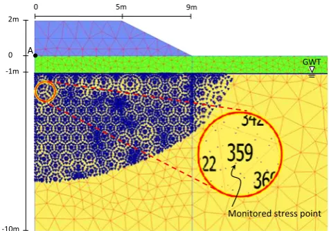
[image:8.595.36.280.56.306.2]

At the end of all analysis 4037 stress points inside the soft soil domain become plastic (seeFig. 5).

Table 9shows the results of the three analyses in terms of total CPU time, total number of required MNR iterations, maximum number of required MNR iterations in one load step, average number of required MNR iterations for all load steps, average value of all residuals for rf, and average value of all residuals for rε.

Similar to the simulations at stress point level, all the timing results presented in this section are also for a PC with Intel Core i7-3820 3.60 GHz processor with the Lahey/Fujitsu FORTRAN Professional V7.3 compiler. The CPU time recorded is for the entire finite element analysis, not just the stress integration part, as this is of more relevance to the design utilisation of numerical models. Comparing the results in Table 9, it can be seen that the duration of FE analysis for Case III is noticeably less than the time required for the other two cases; it is almost 21% shorter than Case I which is remarkable. Case II also results in almost 11% saving in computational cost, compared to Case I. Therefore, it is not surprising to see that overall Case I requires more MNR iterations for stress integration during plastic straining. In addition, while the values GWT

9m 5m 0

2m

0 -1m

-30m

Bothkennar clay Dry crust

[image:8.595.308.546.380.547.2]

Fig. 4.Geometry of the boundary value problem and the idealised soil profile.

[image:8.595.302.552.643.746.2]

Fig. 5.Plastic zone within the soft soil layer, the location of the monitored stress point, and the location of point A for deformation measurement.

Table 9

Results from boundary value level study using S-CLAY1S model with different yield function forms (FTOL¼RTOL¼1E8).

Yield function

CPU time (s)

Total req. MNR iter.

Max. req. MNR iter.

Avg. req. MNR iter.

Avg.rf (fy residual)

Avg.rε

(strain residual)

Case I: usingf1y

681 20,919,493 14 9.19 2.72109

2.921014

Case II: usingf2y

607 18,535,346 13 8.27 2.79109

4.251013

Case III: usingf3y

538 16,319,311 9 6.39 2.65109

1.191012

M. Rezania et al. / Finite Elements in Analysis and Design 90 (2014) 74–83

of bothRTOLand FTOLtolerances are the same, in general after convergence the averager_εresiduals are several orders of magni-tude smaller than averagerf residuals; this indicates that in the

concurrent iterative procedure, the tolerance with regards to the strain residual is always satisfiedfirst, but satisfyingFTOLrequires further iterations in order to achieve the required error control, which subsequently results inr_εgetting substantially smaller than the desiredRTOL.

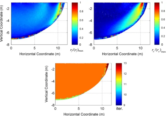
For an enhanced evaluation of the MNR performance with different yield function forms, the error proportionalities within the plastic domain of Fig. 5 are presented in Figs. 6–8 using contour maps of normalised residuals and iteration numbers. It should be mentioned that these contours are plotted at the end of consolidation in each analysis and hence signify values only

at the final time increment of the analyses. However, they still provide a very good graphical glimpse of the return mapping algorithm function in different cases.

From Figs. 6–8it is generally observed that residual contour maps are somehow representing the mobilised slip surface due to loading (particularly in Cases II and III); inFig. 8related to Case III even the stress concentration below the embankment toe can be identified. This could be expected given the fact that stress points along the slip surface are the more critical ones where the imposed stress distribution deviates signi_ficantly from the initial stress distribution in the ground. Case I results in less residual values, i.e. less errors, over the plastic points; however that is accompanied with higher computational cost as in this particular snapshot for the majority of the points 13 stress integration

rf/(rf)max rε/(rε)max

0 0

[image:9.595.124.482.218.460.2]

iter.

Fig. 6.Contour maps for normalised residualsrfandrε, and required number of iterations based onfy1, Case I;ðrfÞmaxis 9.9210

9

andðrεÞmaxis 5.5910

14

.

rf/(rf)max r_ε/(r_ε)_max

0 0

iter.

Fig. 7. Contour maps for normalised residualsrfandrε, and required number of iterations based onfy2, Case II;ðrfÞmaxis 9.9410

9

andðrεÞmaxis 6.6510

13

[image:9.595.130.478.490.732.2]

iterations are needed (seeFig. 6). Towards Case II and Case III the errors become more widely distributed between maximum and minimum amounts (see Figs. 7 and 8), and the required MNR iterations in the plastic domain reduces considerably in Case III.

For further comparison, the abovefinite element analysis has been repeated with tolerance values,RTOLandFTOL, relaxed once to 1106_{and the other time to 110}4_{. For all nine analyses,}

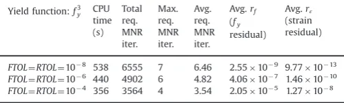
the MNR iteration numbers and the values of residuals were monitored at a single stress point inside element number 359 within the plastic domain (seeFig. 5). The results of all FE analyses are summarised inTables 10–12.

The results from all runs show remarkably consistent trend; indeed, the same observations and conclusions, as those explained above based on the results inTable 9, apply. All analyses display a

“tolerance proportionality” [31] with regards to FTOL; also, the required number of MNR iterations and hence the analysis dura-tion is constantly decreasing from whenf1yis used to whenf

3

y is

used. In addition, it is seen that in each case the timings are largely sensitive to the specified error tolerances. For example, the difference in the CPU time related to the employment of f2_y, between when FTOL¼RTOL¼108_{and whenFTOL¼RTOL¼10}4_,

is more than 34% (seeTable 10). Also significant variations in the number of required MNR iterations is observed, for example when yield function form f3y is used, the average number of required

MNR iterations withFTOL¼RTOL¼104_{is over 45 % less than the}

same iteration number when FTOL¼RTOL¼108 _{(seeTable 11).}

It should be noted that in all nine analyses, settlement has been monitored at the ground surface under the centreline of the embankment (point A in Fig. 5), and in all runs, but one, the predicted displacements have been uniformly matching. The one analysis with dissimilar settlement prediction is related to the employment off3ywithFTOL¼RTOL¼10

4

where thefinal settle-ment has been 0.8 mm less than other FE runs; this appears to be a negligible variance.

5. Conclusion

The robustness of a modified Newton–Raphson algorithm applied to the S-CLAY1S model has been evaluated using different

forms of its yield function. Although the proposed stress update scheme is generally very robust, and impartial in terms of accuracy; however, its convergence performance is found to be

rf/(rf)max rε/(rε)max

0 0

[image:10.595.118.469.57.299.2]

iter.

[image:10.595.303.552.355.433.2]

Fig. 8.Contour maps for normalised residualsrf andrε, and required number of iterations based onf3y, Case III;ðrfÞmaxis 9.97109andðrεÞmaxis 1.981012.

Table 10

Results from boundary value level study using S-CLAY1S model with yield functionf1y.

Yield function:f1y CPU time (s)

Total req. MNR iter.

Max. req. MNR iter.

Avg. req. MNR iter.

Avg.rf (fy residual)

Avg.rε

(strain residual)

FTOL¼RTOL¼108

681 8444 9 8.32 9.93109

1.981014

FTOL¼RTOL¼106

553 6701 8 6.59 3.72107

2.661012

FTOL¼RTOL¼104

538 5359 6 5.27 2.45105

1.881010

Table 11

Results from boundary value level study using S-CLAY1S model with yield functionf2

y.

Yield function:f2

y CPU time (s)

Total req. MNR iter.

Max. req. MNR iter.

Avg. req. MNR iter.

Avg.rf (fy residual)

Avg.rε

(strain residual)

FTOL¼RTOL¼108

607 7520 8 7.42 2.60109

2.161013

FTOL¼RTOL¼106

488 5862 7 5.78 4.00107

3.591011

FTOL¼RTOL¼104 _{399 4505 5 4.43 2.1410}5 _3.11109

Table 12

Results from boundary value level study using S-CLAY1S model with yield functionf3y.

Yield function:f3y CPU time (s)

Total req. MNR iter.

Max. req. MNR iter.

Avg. req. MNR iter.

Avg.rf (fy residual)

Avg.rε

(strain residual)

FTOL¼RTOL¼108

538 6555 7 6.46 2.55109

9.771013

FTOL¼RTOL¼106

440 4902 6 4.82 4.06107

1.461010

FTOL¼RTOL¼104

356 3564 4 3.54 2.05105

1.27108

M. Rezania et al. / Finite Elements in Analysis and Design 90 (2014) 74–83

[image:10.595.303.552.488.565.2] [image:10.595.302.552.621.696.2]

considerably sensitive to the yield function equation as well as acceptable tolerances. There is a particular form of the yield function, i.e.f3y, that results in the smallest number of iterations

and the most robust yield form. Over a simple example it was shown that employment of this form of the S-CLAY1S yield function equation for boundary value level analysis can result in over 20% saving in computational cost which is considerable. This is specifically promising given that the plastic domain in the analysed example was relatively small. Similar form of the yield function for other models can be of particular bene_fit for analysing highly non-linear problems where small load steps produce large strain increments, hence fewer stress update iterations are favour-able to provide an economical measure for integrating elasto-plastic constitutive laws. Overall this paper highlights the possi-bility of using simple numerical techniques to enhance the stress integration algorithm's performance for complex constitutive models particularly those belonging to the critical state family.

Acknowledgements

The work presented was sponsored by the Academy of Finland (Grant 1284594) and the European Community through the programme“People”as part of the Industry-Academia Pathways and Partnerships project GEO-INSTALL (PIAP-GA-2009–230638). Thefirst author would also like to thank thefinancial support from the University of Nottingham's Dean of Engineering award.

References

[1]J. Graham, M.L. Noonan, K.V. Lew, Yield states and stress–strain relationships in a natural plastic clay, Can. Geotech. J. 20 (1983) 502–516.

[2] Y.F. Dafalias, An anisotropic critical state clay plasticity model, in: Proceedings of the Second International Conference on Constitutive Laws for Engineering Materials, Tucson, US, 1987, pp. 513–521.

[3] S.J. Wheeler, M. Karstunen, A. Näätänen, Anisotropic hardening model for normally consolidated soft clay, in: Proceedings of the Seventh International Symposium on Numerical Models in Geomechanics (NUMOG VII), Graz, Austria, 1999, pp. 33–40.

[4]D.K. Kim, Comparisons of constitutive models for anisotropic soils, KSCE J. Civ. Eng. 8 (2004) 403–409.

[5] H., Sekiguchi, H. Ohta, Induced anisotropy and time dependency in clays, in: Proceedings of the Ninth International Conference on Soil Mechanics and Foundation Engineering (ICSMFE), Tokyo, Japan, 1977, pp. 229–238. [6] M.C.R. Davies, T.A. Newson, A critical state constitutive model for anisotropic

soils, in: Proceedings of the Wroth Memorial Symposium: Predictive Soil Mechanics, Thomas Telford, London, 1993, pp. 219–229.

[7]A.J. Whittle, M.J. Kavvadas, Formulation of MIT-E3 constitutive model for overconsolidated clays, J. Geotech. Eng. 120 (1994) 173–198.

[8]S.J. Wheeler, A. Näätänen, M. Karstunen, M. Lojander, An anisotropic elasto-plastic model for soft clays, Can. Geotech. J. 40 (2003) 403–418.

[9]Y.F. Dafalias, M.T. Manzari, A.G. Papadimitriou, SANICLAY: simple anisotropic clay plasticity model, Int. J. Numer. Anal. Meth. Geomech. 30 (2006) 1231–1257.

[10]M. Karstunen, H. Krenn, S.J. Wheeler, M. Koskinen, R. Zentar, The effect of anisotropy and destructuration on thebehaviour of Murro test embankment, Int. J. Geomech. 5 (2005) 87–97.

[11] M. Karstunen, C. Wiltafsky, H. Krenn, F. Scharinger, H.F. Schweiger, Modelling the behaviour of an embankment on soft clay with different constitutive models, Int. J. Numer. Anal. Meth. Geomech. 30 (2006) 953–982.

[12]A. Yildiz, M. Karstunen, H. Krenn, Effect of anisotropy and destructuration on behavior of haarajoki test embankment, Int. J. Geomech. 9 (2009) 153–168. [13]J. Castro, M. Karstunen, Numerical simulations of stone column installation,

Can. Geotech. J. 47 (2010) 1127–1138.

[14]A.J. Abbo, S.W. Sloan, An automatic load stepping algorithm with error control, Int. J. Numer. Meth. Eng. 39 (1996) 1737–1759.

[15]J.C. Simo, R.L. Taylor, Consistent tangent operators for rate-independent elastoplasticity, Comput. Meth. Appl. Mech. Eng. 48 (1985) 101–118. [16]M. Ortiz, J.C. Simo, An analysis of a new class of integration algorithms for

elastoplastic constitutive relations, Int. J. Numer. Meth. Eng. 23 (1986) 353–366.

[17] R.I. Borja, Cam-Clay plasticity, Part II: implicit integration of constitutive equation based on a nonlinear elastic stress predictor, Comput. Meth. Appl. Mech. Eng. 88 (1991) 225–240.

[18]K.H. Roscoe, J.B. Burland, On the generalized stress–strain behaviour of‘wet’ clay, Eng. Plast. (1968) 553–609.

[19] T. Pipatpongsa, M.H. Khosravi, S. Kanazawa, S. Likitlersuang, Effect of the modified Cam-clay yield function's form on performance of the Backward-Euler stress update algorithm, in: Proceedings of the 22nd KKCNN symposium on Civil Engineering, Chiangmai, Thailand, 2009, pp. 509–514.

[20] K.H. Roscoe, A.N. Schofield, A. Thurairajah, Yielding of clays in state wetter than critical, Geotechnique 13 (1963) 211–240.

[21] M.H. Khosravi, T. Pipatpongsa, S. Kanazawa, A. Iizuka, Effect of yield function's form on performance of the Backward-Euler stress update algorithm for the original Cam-clay model, in: Proceedings of the 11th JSCE International Summer Symposium, Tokyo, Japan, 2009, pp. 161–164.

[22] W.M. Coombs, R.S. Crouch, Algorithmic issues for three-invariant hyperplastic Critical State models, Comput. Meth. Appl. Mech. Eng. 200 (2011) 2297–2318. [23] N. Sivasithamparam, Development and implementation of advanced soft soil models infinite elements (Ph.D. thesis), Department of Civil and Environ-mental Engineering, University of Strathclyde, Glasgow, UK, 2012.

[24] A. Gens, R. Nova, Conceptual bases for a constitutive model for bonded soils and weak rocks, in: Proceedings of the International Symposium on Hard Soils–Soft Rocks, Athens, Greece, 1993, pp. 485–494.

[25] M. Koskinen, M. Karstunen, S.J. Wheeler, Modelling destructuration and anisotropy of a natural soft clay, in: Proceedings of the Fifth European Conference on Numerical Methods in Geotechnical Engineering, Paris, France, 2002, pp. 11–20.

[26] K. McGinty, The stress–strain behaviour of Bothkennar clay (Ph.D. thesis), Department of Civil Engineering, University of Glasgow, Glasgow, UK, 2006. [27] M. Karstunen, M. Rezania, N. Sivasithamparam, M. Leoni, Z-Y. Yin, Recent

developments on modelling time-dependent behaviour of soft natural clays, in: Proceedings of the XXV Mexican National Meeting of Soil Mechanics and Geotechnical Engineering, Acapulco, Mexico, 2010, pp. 931–938.

[28] LF Fortran 95 Language Reference, Lahey Computer Systems, Inc.

[29] H.S. Yu, Plasticity and Geotechnics. Advances in Mechanics and Mathematics, Springer, 2006.

[30] R.B.J. Brinkgreve, W.M. Swolfs, E. Engin, PLAXIS 2D Reference manual, Delft University of Technology and PLAXIS b.v., The Netherlands, 2010.