warwick.ac.uk/lib-publications
Original citation:
Dinh, Quang Truong, Marco, James, Greenwood, David, Ahn, Kyoung Kwan and Yoon, Jong Il
(2017) A data-based hybrid driven control for networked-based remote control applications.
In: IEEE International Conference on Mechatronics, Churchill, VIC, Australia, 13–15 Feb 2017
Permanent WRAP URL:
http://wrap.warwick.ac.uk/86206
Copyright and reuse:
The Warwick Research Archive Portal (WRAP) makes this work by researchers of the
University of Warwick available open access under the following conditions. Copyright ©
and all moral rights to the version of the paper presented here belong to the individual
author(s) and/or other copyright owners. To the extent reasonable and practicable the
material made available in WRAP has been checked for eligibility before being made
available.
Copies of full items can be used for personal research or study, educational, or not-for profit
purposes without prior permission or charge. Provided that the authors, title and full
bibliographic details are credited, a hyperlink and/or URL is given for the original metadata
page and the content is not changed in any way.
Publisher’s statement:
© 2017 IEEE. Personal use of this material is permitted. Permission from IEEE must be
obtained for all other uses, in any current or future media, including reprinting
/republishing this material for advertising or promotional purposes, creating new collective
works, for resale or redistribution to servers or lists, or reuse of any copyrighted component
of this work in other works.
A note on versions:
The version presented here may differ from the published version or, version of record, if
you wish to cite this item you are advised to consult the publisher’s version. Please see the
‘permanent WRAP url’ above for details on accessing the published version and note that
access may require a subscription.
A Data-Based Hybrid Driven Control for
Networked-based Remote Control Applications
Truong Quang Dinh, James Marco, David Greenwood
Warwick Manufacturing Group (WMG) University of Warwick
Coventry CV4 7 AL, UK
[email protected],[email protected]
Kyoung Kwan Ahn
School of Mechanical Engineering University of Ulsan Ulsan 680-749, Korea
Jong Il Yoon
KOCETI KOCETI Gunsan 573-540, Korea
Abstract—This paper develops a data-based hybrid driven control (DHDC) approach for a class of networked nonlinear systems compromising delays, packet dropouts and disturbances. First, the delays and/or packet dropouts are detected and updated online using a network problem detector. Second, a single-variable first-order proportional-integral (PI) -based adaptive grey model is designed to predict in a near future the network problems. Third, a hybrid driven scheme integrated a small adaptive buffer is used to allow the system to operate without any interrupt due to the large delays or packet dropouts. Forth, a prediction-based model-free adaptive controller is developed to compensate for the network problems. Effectiveness of the proposed approach is demonstrated through a case study.
Keywords—networked control system; time delays; packet dropouts; prediction; model free; stability
I. INTRODUCTION
Recently with the rapid development of networking technologies, network-based remote control gains more and more attention because of its advantages over wiring control. Time delay (computation delays at the controller and communication delays at the forward and backward channels) and packet dropout are two important and unavoidable factors existing in any networked control system (NCS) [1], [10].
To address stability of NCSs with communication delays, many studies were carried out in which the controller designs were depended on the assumptions, that the time delay was constant or bounded [2], had a probability distribution function [3], or based on time delay analyses [4]. In other studies, control concepts based on variable sampling periods using neural network or prediction theories were adopted for NCSs with large delays [5]. Although the favorable results were achieved, the observation of real delay data to train and construct the NCSs was not appropriately discussed.
For NCSs compromising both time delays and packet dropouts, many important methodologies, such as predictive control [6], adaptive control [7], hybrid control [8], and robust control [9],[10], were proposed in which delays and packet dropouts were assumed to be priorly known and bounded. Another trend is known as control based on efficient networks with compensation strategy [11]. However, their applicability
may be limited due to the complex network designs. As a feasible solution for these problems, a robust variable sampling period control approach tagged RVSPC [12] has been proposed. Some limitations still exist in the RVSPC as: the state feedback control unit is basically designed for a well-defined networked linear system which is actually not easy to be achieved; for a NCS with large delays and/or high packet dropout ratio, the performance may be degraded when the driving commands and sensing signals are long delayed/dropped. Thanks to the development of model-free control, this advanced technology is successful utilized to construct NCSs with the good adaptability [13]. Nevertheless, these control schemes remain some open problems: the network problems are assumed to be bounded within a pre-defined maximum round trip delay; the large delay bound also leads to the slow convergence speed; the buffers need to be large enough to deal with the worst network states; the task must be given at the plant side while it is normally at the control side in actual remote applications.
This paper aims to address all the problems raised by [12], [13] by introducing a data-based hybrid driven control (DHDC) approach for a class of imperfect NSCs. The main contribution of this work can be expressed as:
1) Delays and packet dropouts are quickly and accurately detected online by a network problem detector (NPD) using a new concept to classify network problems.
2) A single-variable first-order PI-based adaptive grey model (PIAGM(1,1)) is more generally designed for a capable of forecasting precisely in a near future the network problems. 3) A hybrid driven scheme integrated a small adaptive buffer (SAB) is developed to operate the system smoothly. The buffer size is online optimized based on the estimated packet dropouts and subsequently, simplifies the control design. 4) A prediction-based model-free adaptive controller (PMFAC) is then constructed to compensate for the small delays and packet dropouts. By employing the hybrid driven scheme and SAB, a so-calledsk-step-ahead control technique is used to produce a dynamic vector of the control inputs according to the buffer size.
II. PROBLEMDESCRIPTION
An output y of a generic discrete-time nonlinear system with non-uniform sampling states can be described as:
( 1) ( ( ),..., ( y), ( ),..., ( U))
y k f y k y k l U k U k l (1) wherekdenotes the time stamp at working stepkth; y k( )R1;
( ) mu
U k R is the control input vector; f(*) is an unknown nonlinear function;lyandluare unknown orders.
To build the free-model adaptive control (MFAC) for system (1), two following assumptions are made [13].
Assumption 1: the partial derivative of function f(*) in (1) with respect to the control inputu(k) is continuous.
Assumption 2: there is a positive constantbsuch that system (1) is generalized Lipschitz, y k
1
b U k
, for anyk,
1
1
,
1
0y k y k y k U k U k U k
.
Based on Assumptions 1 and 2, system (1) can be represented in a compacted form dynamic linearization [13]
( 1) T( ) ( )
y k k U k
(2)
The incremental control algorithm is derived for system (1) using the MFAC [13] as follows:
2
( 1)
ˆ( ) ˆ( 1) ( ) ˆ ( 1) ( 1)
( 1)
T U k
k k y k k U k
U k
(3)
ˆ( ) , or ( 1) ˆ( ) ˆ(0)
ˆ ˆ
( ( )) ( (0)) ( ( ) { ( )}; ( ) { ( )}; 1,..., )
i i
i i
i i
i i u
k u k
k
sign k sign
U k u k k k i m
(4)
2ˆ
1 ,
ˆ
r k
U k G k y k y k G k
k
(5)
whereˆi( )k is the estimation ofi( )k with initial value
ˆ(0)
i
; , are the step-sizes normally set within (0,1] ; ,
are the weight factors; is a small positive constant;
yr(k+1) is the reference ofy(k).
Definition 1:the problems in a network are defined as:
The communication delays in both forward and/or backward channels are denoted acaandsc. Correspondingly, two threshold values,caandsc, are defined to classify small and large communication delays. Large delays are treated as packet dropouts:
( ) or ( ) Smalldelay
( ) or ( ) Packet dropout
ca ca sc sc
ca ca sc sc
k k
k k
(6)
A packet disorder is also considered as a packet dropout.
“Virtual” switches,ScaandSsc, are in turn used to represent the packet dropouts in the forward and backward channels.
Sca(Ssc) is opened (or 1) once a packet dropout event exists.
A set of continuous packet dropouts at time stamp k is denoted aspca(k) orpsc(k).
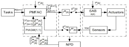
[image:3.595.321.547.53.136.2] The computation delay,com, is bounded,com( )k com.
Fig. 1. A generic NCS architecture using the proposed DHDC approach.
III. DATA-BASEDHYBRIDDRIVENCONTROLAPPROACH A generic NCS using the DHDC is depicted in Fig. 1 in which the tasks consist of a main task to control the plant (1) and other tasks, which cause computation delays.
Remark 1:The DHDC approach is developed for system (1) over an imperfect network with following issues:
The NPD is used to detect and classify the network problems using Definition 1.
The PIAGM(1,1) with prediction step sizesk uses the NPD outputs to predict the network problems in a near future.
Both the controller, sensors and actuators are hybrid time-event-driven. Event driven is activated once small delays are detected; otherwise, time driven is activated.
The PMFAC is designed to compensate for small delays and packet dropouts. According to the sk-step-ahead prediction, a vector of control inputs are derived and the SAB buffer at the plant side is used to drive the actuators.
A. NPD Detector
Remark 2: The hardware, PIC18F4620 MCU (from Microchip) equipped with the 4-MHz oscillator, and the embedded time stamp-based detection logics developed in [12] are used to build the NPD. Thus, the real-time measurement accuracy is 50s.
From Remark 2 and using Definition 1, for each working step, the NPD detects accurately the current network states with a delay set,ca( ),k sc( )k andcom( )k , and a set of continuous packet dropouts,pca(k) andpsc(k).
B. PIAGM(1,1) Predictor and Hybrid Driven Method Remark 3:Grey model is known as a feasible tool for online prediction while requiring only a few historical data [12],[14]. The PIAGM(1,1) is designed as the followings:
The model is developed a more efficient way using simple PI algorithm and neural network.
It is capable of forecasting any random time-series data by using a simple data conversion with additive factors.
The robust prediction is guaranteed by Lyapunov condition. From Remark 1, the PIAGM(1,1) is employed to perform the sk-step-ahead prediction of the network problems: delays,ˆca( )
s
k i
ˆsc( ) andˆcom( ),
s s
k i k i
and packet
dropouts,pˆca(k i s) andpˆsc(k i s)in which is=2,...,sk, sk is the smallest value corresponding to a case:
ˆ ˆ ˆ
For a step (k+1)th, using Definition 1 and PIAGM(1,1) outputs, the hybrid time-event driven method can be expressed through dynamic sampling rates,TC(k+1) andTA(k+1), which are derived for the controller side and plant side, respectively:
ˆ ˆ ˆ
1 1 min 1 , min 1 ,
ˆ ˆ ˆ
1 min , 1 min 1 ,
C com ca ca sc sc
A sc sc com ca ca
T k k k k
T k k k k
(7)
C. SAB Buffer
To eliminate packet dropout effect, the SAB is utilized at the plant side. The key concept here is to regulate online the buffer size, b(k+1), to store enough commands to drive the actuators for ˆca( )
k
p k s continuous packet dropouts.
Algorithm 1SAB-based Control Procedure
Step 1: Set the initial size of the SAB,b(0)= bmin= 2; Step 2: For step (k+1)that the controller side, base on the s
k -step-ahead prediction using the PIAGM(1,1): set b(k+1) = sk and, correspondingly, generate a set of time-stamped control inputs,{ ( 1),..., (k s )}
k
U k t U t , using the PMFAC; Step 3: For step (k+1)that the plant side:
If a new package sent from the controller is arrived: + Re-size the SAB with the new sizeb(k+1)
+ Update the new control inputs and store in the SAB
Extract data from the SAB to drive the actuators.
D. PMFAC Controller
As the main control unit, the PMFAC takes part in driving the actuators to reach the desired target based on Remark 1:
For each step defined by the hybrid time-event driven method (TC(k)) and based on the PIAGM(1,1) output,s
k, a set of the control inputs are generated for the nextsksteps using an iterative estimation scheme.
A time delay factor is invoked into the controller design process to compensate for this problem.
IV. PIAGM(1,1) PREDICTOR
A. PIAGM(1,1) Design
Remark 4:For any random data set of the predicted object,
yobj, it can be converted into a Grey sequence satisfying both the Grey checking conditions using the cubic spline interpolation (called as SP) and two non-negative smart additive factors,c1andc2, derived by Theorem 1 in [12].
Prediction procedure for an object,yobj, can be expressed as:
Algorithm 2PIAGM(1,1) Model to Predict An Objectyobj Step 1: For an object with a data sequence
1
{ ( ),..., ( )}( 4)
obj obj O obj Om
Y y t y t m , the raw input grey
sequence,Yraw{yraw( ),...,t1 yraw( )}(tn n4) , is derived as
1
(0)( ) 0 ( ) (1 0) ( , ), 1,...,
raw i i obj i i obj i
y t y t SP Y t i n (8) where 0
i
is an activated factors based on Remark 4; The input grey sequence is computed as
0 0 0 0
1 2
{ ( ), ( ),..., ( )} 0;n 4
y y t y t y t n (9)
where 0
1 2
( )i raw( )i ;
y t y t c c
Step 2: Generate a new seriesy(1)by generating fromy(0):
1
1 21 , 1,...,
k
k i obj i i
y t
y t c c t k n (10) Step 3: Create the background seriesz(1)fromy(1)as 1
1
1
2
1
1 ; 2,...,
k k k k k
z t w t y t w t y t k n (11)
where
1
, 2
k k
w t w t is a set of weight factors computed as
1 1 1 2 2
1
2 1 1 2 1 2
( ) 0.5 1 ( ) 1 1 ( )
( ) 0.5 1 1 ( ) 1 ( )
A A
k k k
A A
k k k
w t w t w t
w t w t w t
(12)
where 0 A( ) 1
k
w t
is an adaptive factor; { , 1 2} are:
0 0 1 1 0 0 1 2 1 1{1,0}, IF : ;
{ , } {1,1}, IF : ;
{0,1},Others;
raw k k raw k obj k raw k obj k raw k k
y t SP t y t y t
y t y t y t SP t
(13)
Step 4: Establish the grey differential equation 0
1
k k
y t az t b (14)
By employing the least square estimation [12], one has:
1
ˆ
ˆ ˆ T ( T ) T ab a b B B B Y
(15)
1 0 2 2 1 0 1 , ; 1 n nz t y t
B Y
z t y t
Step 5: The PIAGM(1,1) prediction is then setup as:
0
1 2
1
11
ˆ ˆ ( ) ( )
ˆ ;
ˆ
1 ( )
k k k k
k k
b a w t w t y t y t
w t a t
(16)
Step 6: Produce the sk-step-ahead prediction yobj (at step (k+sk)th)based on (9) and (16):
0
0
0
1 2
ˆ ˆ ˆ .
k k
obj k raw k s k s
y k s y t y t c c (17)
B. Prediction Stability Analysis
A PI-based neural network (PINN) controller with three layers is designed to regulate the ‘control input’ A( )
k
w t . The input layer is the prediction error sequence{ ( )}withP
i k
e t
0 ˆ 0
( ) ( ) ( )
P
i k raw k n i raw k n i
e t y t y t . The hidden layer has two nodes P and I following PI algorithm and the output layer to compute the adaptive factor A( )
k
w t in (12). Define { P( ), I( )}
i k i k
w t w t is a weight vector of the hidden nodes with respect to inputithand{ P( ), I( )}
k k
w t w t is a weight vector of the output layer. Since, the output from each hidden node is derived in (18) while the network output is derived in (19):
1
1
( ) ( ) ( ) : Node P
( ) ( 1) ( ):Node I
n
P P P
k i i k i k n I I I P
k k i i i k
O t w t e t
O t O t w e t
(18) 1( ) (1 ( )) ,
( ) ( ) ( ) ( ) ( ).
NN
O A
k k
NN P P I I k k k k k
w t e t
O t w t O t w t O t
A prediction error function is defined as
2 1
( ) 0.5 n ( ( )) .
P P
k i i k
E t e t
(20)The weight factors of the PINN controller are online tuned using the back-propagation algorithm as
/ / /
/ / /
( 1) ( ) ( ) ( ) / ( )
( 1) ( ) ( ) ( ) / ( )
P I P I P P I k k P k k k P I P I P P I i k i k P k k i k
w t w t t E t w t
w t w t t E t w t
(21)
where P( )tk is the learning rate within range (0,1]; the other
factors in (21) are derived using the partial derivative of the error function with respect to each weight.
Theorem 1: By selecting the learning rateP( )tk to satisfy
(22), the stability of the PIAGM(1,1) prediction is guaranteed.
1 2
1 ( ) ( ) 0.5 ( ) ( ) 0
n P
i k k k P k i e t F t F t t
(22)1
( ) ( ) ( ) ( )
( ) .
( ) ( ) ( ) ( )
P P P P n
j k k j k k
k P P I I
j i k j k i k j k
e t E t e t E t
F t
w t w t w t w t
Proof: Define a Lyapunov function as (23). The theorem can be then proofed by using the same method in [21].
21
( ) 0.5 n .
P P
k i i k
V t e t
(23)V. PMFAC CONTROLLER
A. PMFAC Design
Remark 5: For the networked system (1) with problems defined using Definition 1, the PMFAC is built based on the PIAGM(1,1) prediction results to produce the control input. Thus, the last plant information received at the controller side can be described asy k*( ) y k( tk):
Case 1- there is only a delaysc( )k and no packet dropout in
the backward channel at the current step, tk sc( )k ;
Case 2– currently, there existicontinuous packet dropouts in the backward channel, k sc k A( )
j k i
t T j
.Based on Remarks 1 and 5, the control problem is now simplified to design a set of control inputs{ (U ki)}(for Algorithm 1) at steps{(ki)}in whichiis defined as
1
1 2
ˆ ˆ
( ( 1) ( 1))
( ), 2
com ca
i A
i j k
t k k
T k i i s
(28)Algorithm 3Control Input Calculation Using PMFAC
Step 1: Compute the control input for step (k1)th:
* 1
( ) ( )( (r ) ( ))
U k G k y k y k
(29)
Step 2: Using (3) to (5), compute the set of control inputs { (U ki)},i2,...,skusing iterative method (00):
1
ˆ
( ) T( ) ( )
i i
y k k U k
(30)
1
( ) ( )( (r ) ( ))
i i i
U k G k y k y k
(31)
1
( i ) ( i) ( i)
U k U k U k (32)
B. Control Stability Analysis
Lemma 1[25]: Consider the following linear system:
( 1) ( ) ( ) ( ),0
( ) ( ), , 1,...,0
k k
x k x k k x k
x k k k
(33)
where x(k) is the scalar state, ( )k is the time-varying parameter, and( )k is the initial condition.
System (32) is asymptotically stable if0( ) 2(2k 1)1.
Proof:Selecting the Lyapunov function as [25]
1
2
V k V k V k (34)
2
1 1 2
1 ; 2
k x i j k i
V k px k V k
q jwherepandqare positive scalars,x2
k ( ) (k x kk). By taking the change of this Lyapunov function and defined
[ ( ) ( k)]TX k x k x k , bellow relation is obtained [13]:
1
T
V k V k V k X k X k
(35)
2 2
( )
( ) ( ) ( )
q p k q
p k q p q k q
The system is asymptotically stable onceV k
0. This lead to the inequalities in (35), 0. By applying the Schur complement lemma [12], following condition is achieved:
2 2 2
1
10 k 2pq pq p q 2 1 2 (36) The requirement (36) to ensure the stability of system (33), therefore, completes the proof.
From (28), it is clear thatiis definitely bounded for each working step,1isk. The following is to carry out the
stability analysis for the system at stepk*(ksk).
Theorem 2: By selecting the weight factor
2 2 22 1 /16
k
s b
, the networked control of system (1) is guaranteed to be stable with zero steady state tracking error for a constant reference ofy,yr=const.
Proof: Applying the PMFAC for the networked control of system (1), the tracking error with outputyis derived as
* r
* r
* 1
ˆT
* 1 .
e k y y k y y k k U k (37)
Replacing (31) into (37) and using (5), one has:
* * 1 1
ˆT
ˆ ( || ( ) || )ˆ 2 1
; ore k e k k k k (38)
*
1 ˆ
2( || ( ) || )ˆ 2 1 sk.e k e k k k
(39)
Taking the change of control error, one has:
*
* 1
T
* ; ore k y k k U k
(40)
2 *
2
ˆ
1 .
ˆ
k
s
T
k
e k e k k G k
k
Comparing (41) with Lemma 1, the system is stable with zero steady state tracking error only if:
2 2
ˆ ˆ ˆ 2
0 1 .
2 1
ˆ ˆ
k
k
s
T T
s
k k k k
k k
(42)
Based on the reset algorithm (4), without loss of generality,
k is assumed to be positive for all the time. It is clear that:
2 1ˆ ˆ ˆ
1 1.
k
s
T k k k
(43)
From Assumption 1 and (2), following relation is obtained:
2
1
ˆ
0
2
ˆ ˆ ˆ
T k k b b
k k k
(44)
From (42) to (44), to ensure the system stability, one has:
2 2 2
/ (2 ) 2 / (2 sk 1) (2 sk 1) /16
b b
(45)
The relation (45), therefore, completes the proof.
VI. CASESTUDY
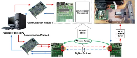
A. Problem and Hardware Setup
[image:6.595.41.288.67.300.2]Here, the network setup and DC servomotor system in [12] were used to carry out a comparative study on the motor speed tracking control (see Fig. 2). A comparative between the proposed DHDC approach and existing model-based and model-free methods has been considered. Two model-based methods were employed which were the robust variable sampling period controller (RVSPC) [12], and the static state feedback controller (SSFC) [10] combined with the NPD module and a fixed buffer, tagged as SSFC-FB. A model-free method - the MFAC [13] with fixed weight factor combined with a fixed buffer (named as MFAC-FB) was used to perform the comparison.
Fig. 2. Configuration of the networked servomotor control system.
B. Setting of Controller Parameters
To design the RVSPC and SSFC-FB, the system plant needed to be known. In this case, it was well addressed in [12]
1
x k Ax k Bu k Ed k
y k Cx k
235870 4934200 1 0
, , .
1 0 0 32298000
T
A B C
The RVSPC control gains were derived in [12]. The SSFC-FB gains KSSFC FB
0.3652 0.2539
were achieved by considering the total delay as d 0.1 .SSFC s
Its buffer size was fixed as 5. For the DHDC scheme, using Definition 1, the delay threshold values are selected as:
0.025 ; 0.035
com s ca s
; andsc 0.035s. The controller was then constructed without using the linearized plant:
5
ˆ ˆ
1, 1, 1, (0) (0) 2, 10 , 0 6.5.
For the
MFAC-FB, the buffer size was also fixed as 5. The control parameters were set as1,1, 1, (0)ˆ ˆ(0) 2,
5
10 , 20.5
corresponding to the worst network state.
C. Experiments and Discussions
Computation delays in [12] and two disturbance sources were added to create the control challenges. The first disturbance came as the magnetic load applied to the motor shaft while the second one was added to the system feedback speed after 12 seconds:
( ) Rand ( )N Nsin(2 N ) 1
N t t A f t
hereANwas given randomly from 0.5 to 1;fNwas varied from 1 to 5 Hz; RandNwas a noise with power 0.005.
[image:6.595.46.281.491.591.2]0 5 10
S
p
ee
d
[r
ad
/s
]
Reference Speed; SSFC-FB;
RVSPC; DHDC
MFAC-BF
0 5 10 15 20 25 30
-0.4 0.0 0.4 0.8
SSFC-FB; RVSPC; MFAC-FB; DHDC
E
rr
or
[r
a
d/
s]
PC Time [s]
[image:7.595.38.288.52.546.2]Added 2nd disturbance souce at T=15s
Fig. 3. Step tracking: performances comparison.
0 5 10 15 20 25 30
0.00 0.02 0.04 0.00 0.01 0.02 0.03
Computation Delay; Estimated Delay
D
e
la
y
[s
]
0.00 0.02
0.04 Network - Forward Delay (C-A); Estimated Delay
D
e
la
y
[s
]
PC Time [s]
Network - Feeback Delay (S-C); Estimated Delay
D
el
a
y
[s
]
0
1 Packet Dropouts; Estimated Packet Dropouts
P
ac
ke
tD
ro
po
ut
s
Fig. 4. Step tracking: one-step-ahead prediction of the delays and forward packet dropouts using the PIAGM(1,1).
0 5 10 15 20 25 30
0 5 10 15 20
Added 2nd disturbance souce at T=15s
S
p
ee
d
[r
a
d/
s]
PC Time [s] Reference Speed
SSFC-FB RVSPC MFAC-FB DHDC
Fig. 5. Multi-step tracking: performance comparison.
0 5 10 15 20 25 30
0.00 0.02 0.04 0.00 0.01 0.02 0.03
Computation Delay; Estimated Delay
D
e
la
y
[s
]
0.00 0.02
0.04 Network - Forward Delay (C-A); Estimated Delay
D
e
la
y
[s
]
PC Time [s]
Network - Feeback Delay (S-C); Estimated Delay
D
el
a
y
[s
]
0
1 Packet Dropouts; Estimated Packet Dropouts
P
ac
ke
tD
ro
po
ut
s
Fig. 6. Multi-step tracking: one-step-ahead prediction of the delays and forward packet dropouts using the PIAGM(1,1).
TABLEI. NCS PERFORMANCESUSINGDIFFERENTCONTROLLERS
Controller
Step responses Percent of
Overshoot [%] Time [s]Settling
Steady State Error [%]
[15~30s]
Mean Square Error [rad/s]2
10-2[15~30s]
SSFC-FB 0.35 1.65 9.07 30.73
RVSPC 0.45 0.95 6.01 4.71
MFAC-FB 0.38 1.36 8.44 21.88
DHDC 0.44 0.66 2.07 2.81
Secondly, the comparative experiments were done for a multi-step speed tracking control profile. The results were then obtained in Fig. 5 and Fig. 6. These results again show the best performance was achieved by using proposed control method. This comes as no surprise, since the proposed method possesses both the optimal design of SAB and the prediction-based adaptive controller, of which the performance is guaranteed by the robust stability constrains.
VII. CONCLUSIONS
This paper presents the advanced data-based hybrid driven control approach for NCSs. The robust tracking performance is theoretically proved and ensured by tuning online the control weight factor according to the estimated network problems. The capability of the proposed DHDC control scheme has been validated through real-time experiments on the networked servomotor system.
ACKNOWLEDGEMENT
This research are supported by: the Engineering and Physical Science Research Council (EPSRC, EP/P511432/1); Innovate UK through the Off-Highway Intelligent Power Management (OHIPM, 49951-373148) in collaboration with the WMG Centre High Value Manufacturing (HVM), JCB and Pektron; and the Koera’s Small and Medium Business Administration (SMBA , S2428274).
REFERENCES
[1] J. Qiu, H. Gao, and S. X. Ding, “Recent Advances on Fuzzy-Model-Based Nonlinear Network Control Systems: A Survey,”IEEE Trans. Ind. Electron., vol. 63, no. 2, pp. 1207-1217, Feb. 2016.
[2] D. Tian, D. Yashiro, and K. Ohnishi, “Wireless Haptic Communication Under Varying Delay by Switching-Channel Bilateral Control With Energy Monitor,”IEEE/ASME Trans. Mechatronics, vol. 17, no. 3, pp. 488-498, Jun. 2012.
[3] F. Yang, Z. Wang, Y. S. Hung, and G. Mahbub, “H∞ control for
networked control systems with random communication delays,”IEEE Trans. Autom. Control, vol. 51, no. 3, pp. 511-518, Mar. 2006. [4] C. C. Choi and W. T. Lee, “Analysis and Compensation of Time Delay
Effects in Hardware-in-the-Loop Simulation for Automotive PMSM Drive System,”IEEE Trans. Ind. Electron., vol. 59, no. 9, pp. 3403-3410, Sep. 2012.
[5] L. L. Chien and L. H. Pau, “Design the remote control system with the time-delay estimator and the adaptive Smith predictor,” IEEE Trans. Ind. Informat., vol. 6, no. 1, pp. 73-80, Feb. 2010.
[6] Z.-H. Pang, G.-P. Liu, D. Zhou, and M. Chen, “Output Tracking Control for Networked Systems: A Model-Based Prediction Approach,”IEEE Trans. Ind. Electron., vol. 61, no. 9, pp. 4867-4877, Sep. 2014. [7] P. Ignaciuk, “Nonlinear Inventory Control With Discrete Sliding Modes
in Systems With Uncertain Delay,”IEEE Trans. Ind. Informat., vol. 10, no. 1, pp. 559-568, Feb. 2014.
[8] A. Baños, F. Perez, and J. Cervera, “Network-Based Reset Control Systems With Time-Varying Delays,”IEEE Trans. Ind. Informat., vol. 10, no. 1, pp. 514-522, Feb. 2014.
[9] H. Gao, T. Chen, and J. Lam, “A new delay system approach to network-based control,”Automatica, vol. 44, no. 1, pp. 39-52, Jan. 2008. [10] H. Li, Z. Sun, M.-Y. Chow, and F. Sun, “Gain-Scheduling-Based State Feedback Integral Control for Networked Control Systems,” IEEE Trans. Ind. Electron., vol. 58, no. 6, pp. 2465-2472, Jun. 2011. [11] H. Li and Y. Shi, “Network-Based Predictive Control for Constrained
Nonlinear Systems with Two-Channel Packet Dropouts,” IEEE Trans. Ind. Electron., vol. 61, no. 3, pp. 1574-1582, Mar. 2014.
[12] D. Q. Truong and K. K. Ahn, “Robust Variable Sampling Period Control for Networked Control Systems,”IEEE Trans. Ind. Electron., vol. 62, no. 9, pp. 5630-5643, Sep. 2015.
[13] Z. H. Pang, G. P. Liu, D. Zhou, and D. Sun, ‘Data-Based Predictive Control for Networked Nonlinear Systems with Network-Included Delay and Packet Dropout,’ IEEE Trans. Ind. Electron., vol. 63, no. 2, pp. 1249-1257, Jan. 2016.
[image:7.595.40.285.543.615.2]