Conjugacy properties of time evolving Dirichlet and gamma random measures

warwick.ac.uk/lib-publications

Original citation:

Papaspiliopoulos, Omiros, Ruggiero, Matteo and Spanò, Dario. (2016) Conjugacy properties of

time-evolving Dirichlet and gamma random measures. Electronic Journal of Statistics, 10 (2). pp.

3452-3489.

Permanent WRAP url:

http://wrap.warwick.ac.uk/83897

Copyright and reuse:

The Warwick Research Archive Portal (WRAP) makes this work of researchers of the University of

Warwick available open access under the following conditions.

This article is made available under the Creative Commons Attribution 2.5 Licence (CC BY 2.5)

and may be reused according to the conditions of the license. For more details see:

https://creativecommons.org/licenses/by/2.5/legalcode

A note on versions:

The version presented in WRAP is the published version, or, version of record, and may be

cited as it appears here.For more information, please contact the WRAP Team at:

Vol. 10 (2016) 3452–3489 ISSN: 1935-7524

DOI:10.1214/16-EJS1194

Conjugacy properties of time-evolving

Dirichlet and gamma random measures

Omiros Papaspiliopoulos∗

ICREA and Department of Economics and Business Universitat Pompeu Fabra

Ram´on Trias Fargas 25-27, 08005, Barcelona, Spain e-mail:[email protected]

Matteo Ruggiero†

Collegio Carlo Alberto and ESOMAS Department University of Torino

C.so Unione Sovietica 218/bis, 10134, Torino, Italy e-mail:[email protected]

and

Dario Span`o

Department of Statistics University of Warwick Coventry CV4 7AL, UK e-mail:[email protected]

Abstract: We extend classic characterisations of posterior distributions under Dirichlet process and gamma random measures priors to a dynamic framework. We consider the problem of learning, from indirect observations, two families of time-dependent processes of interest in Bayesian nonpara-metrics: the first is a dependent Dirichlet process driven by a Fleming–Viot model, and the data are random samples from the process state at discrete times; the second is a collection of dependent gamma random measures driven by a Dawson–Watanabe model, and the data are collected accord-ing to a Poisson point process with intensity given by the process state at discrete times. Both driving processes are diffusions taking values in the space of discrete measures whose support varies with time, and are stationary and reversible with respect to Dirichlet and gamma priors re-spectively. A common methodology is developed to obtain in closed form the time-marginal posteriors given past and present data. These are shown to belong to classes of finite mixtures of Dirichlet processes and gamma random measures for the two models respectively, yielding conjugacy of these classes to the type of data we consider. We provide explicit results on the parameters of the mixture components and on the mixing weights, which are time-varying and drive the mixtures towards the respective priors in absence of further data. Explicit algorithms are provided to recursively compute the parameters of the mixtures. Our results are based on the pro-jective properties of the signals and on certain duality properties of their projections.

∗_{Supported by the MINECO/FEDER via grant MTM2015-67304-P.}

†_{Supported by the European Research Council (ERC) through StG “N-BNP” 306406.}

62G05, 60J60, 60G57.

Keywords and phrases:Bayesian nonparametrics, Dawson–Watanabe process, Dirichlet process, duality, Fleming–Viot process, gamma random measure.

Received December 2015.

Contents

1 Introduction . . . 3453

1.1 Motivation and main contributions . . . 3453

1.2 Hidden Markov models . . . 3457

1.3 Illustration for CIR and WF signals . . . 3458

1.4 Preliminary notation . . . 3462

2 Hidden Markov measures . . . 3463

2.1 Fleming–Viot signals . . . 3463

2.1.1 The static model: Dirichlet processes and mixtures thereof3463 2.1.2 The Fleming–Viot process . . . 3464

2.2 Dawson–Watanabe signals . . . 3466

2.2.1 The static model: Gamma random measures and mixtures thereof . . . 3466

2.2.2 The Dawson–Watanabe process . . . 3467

3 Conjugacy properties of time-evolving Dirichlet and gamma random measures . . . 3468

3.1 Filtering Fleming–Viot signals . . . 3468

3.2 Filtering Dawson–Watanabe signals . . . 3471

4 Theory for computable filtering of FV and DW signals . . . 3474

4.1 Computable filtering and duality . . . 3474

4.2 Computable filtering for Fleming–Viot processes . . . 3477

4.3 Computable filtering for Dawson–Watanabe processes . . . 3480

Acknowledgements . . . 3486

References . . . 3486

1. Introduction

1.1. Motivation and main contributions

In the context of this article, the most relevant strand of this literature attempts to build time evolution into standard random measures for semi-parametric time-series analysis, combining the merits of flexible exchangeable modelling afforded by random measures with those of mainstream generalised linear and time series modelling. For the case of Dirichlet processes, the ref-erence model in Bayesian nonparametrics introduced by Ferguson (1973), the time evolution has often been built into the process by exploiting its celebrated stick-breaking representation (Sethuraman,1994). For example, Dunson (2006) models the dependent process as an autoregression with Dirichlet distributed innovations, Caron et al. (2008) models the noise in a dynamic linear model with a Dirichlet process mixture, Caron et al. (2007) develops a time-varying Dirichlet mixture with reweighing and movement of atoms in the stick-breaking representation, Rodriguez and ter Horst (2008) induces the dependence in time only via the atoms in the stick-breaking representation, by making them into an heteroskedastic random walk. See also Caron and Teh (2012); Caron et al. (2016); Griffin and Steel (2006); Gutierrez et al. (2016); Mena and Ruggiero (2016). The stick-breaking representation of the Dirichlet process has demon-strated its versatility for constructing dependent processes, but makes it hard to derive any analytical information on the posterior structure of the quantities involved. Parallel to these developments, random measures have been combined with hidden Markov time series models, either for allowing the size of the la-tent space to evolve in time using transitions based on a hierarchy of Dirich-let processes, e.g. Beal et al. (2002); Van Gael et al. (2008); Stepleton et al. (2009); Zhang et al. (2014), or for building flexible emission distributions that link the latent states to data, e.g. Yau et al. (2011); Gassiat and Rousseau (2016).

From a probabilistic perspective, there is a fairly canonical way to build sta-tionary processes with marginal distributions specified as random measures us-ing stochastic differential equations. This more principled approach to buildus-ing time series with given marginals has been well explored, both probabilistically and statistically, for finite-dimensional marginal distributions, either using pro-cesses with discontinuous sample paths, as in Barndorff-Nielsen and Shephard (2001) or Griffin (2011), or using diffusions, as we undertake here. The relevance of measure-valued diffusions in Bayesian nonparametrics has been pioneered in Walker et al. (2007), whose construction naturally allows for separate control of the marginal distributions and the memory of the process.

The statistical models we investigate in this article, introduced in Section 2, can be seen as instances of what we call hidden Markov measures, since the models are formulated as hidden Markov models where the latent, unobserved signal is a measure-valued infinite-dimensional Markov process. The signal in the first model is the Fleming–Viot (FV) process, denoted{Xt, t≥0}on some state

space Y (also called type space in population genetics), which admits the law of a Dirichlet process onY as marginal distribution. At timestn, conditionally

onXtn=x, observations are drawn independently fromx, i.e.,

Ytn,i|x iid

parametric model for unknown distributions of Ferguson (1973) and Antoniak (1974). The signal in the second model is the Dawson–Watanabe (DW) process, denoted{Zt, t≥0}and also defined onY, that admits the law of a gamma

ran-dom measure as marginal distribution. At times tn, conditionally onZtn =z,

the observations are a Poisson processYtn on Y with random intensity z, i.e.,

for any collection of disjoint setsA1, . . . , AK∈ Y andK∈N,

Ytn(Ai)|zind∼ Po(z(Ai)).

Hence, this is a time-evolving Cox process and can be seen as a dynamic exten-sion of the classic Bayesian nonparametric model for Poisson point processes of Lo (1982).

The Dirichlet and the gamma random measures, used as Bayesian nonpara-metric priors, have conjugacy properties to observation models of the type described above, which have been exploited both for developing theory and for building simulation algorithms for posterior and predictive inference. These properties, reviewed in Sections2.1.1and2.2.1, have propelled the use of these models into mainstream statistics, and have been used directly in simpler models or to build updating equations within Markov chain Monte Carlo and variational Bayes computational algorithms in hierarchical models.

In this article, for the first time, we show that the dynamic versions of these Dirichlet and gamma models also enjoy certain conjugacy properties. First, we formulate such models as hidden Markov models where the latent signal is a measure-valued diffusion and the observations arise at discrete times according to the mechanisms described above. We then obtain that the filtering distribu-tions, that is the laws of the signal at each observation time conditionally on all data up to that time, are finite mixtures of Dirichlet and gamma random measures respectively. We provide a concrete posterior characterisation of these marginal distributions and explicit algorithms for the recursive computation of the parameters of these mixtures. Our results show that these families of finite mixtures are closed with respect to the Bayesian learning in this dynamic frame-work, and thus provide an extension of the classic posterior characterisations of Antoniak (1974) and Lo (1982) to time-evolving settings.

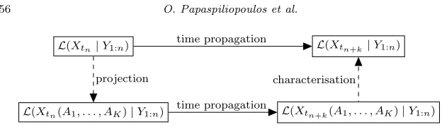
Fig 1_{. Scheme of the general argument for obtaining the filtering distribution of hidden}

Markov models with FV and DW signals, proved in Theorems 3.1 and 3.2. In this figure Xt is the latent measure-valued signal. Given dataY1:n, the future distribution of the

sig-nalL(Xtn+k |Y1:n)at timetn+k is determined by taking its finite-dimensional projection

L(Xtn(A1, . . . , AK) |Y1:n) onto an arbitrary partition (A1, . . . , AK), evaluating the

rela-tive propagationL(Xtn+k(A1, . . . , AK)|Y1:n)at timetn+k, and by exploiting the projective

characterisation of the filtering distributions.

Then we exploit the fact that the dynamics of these finite-dimensional distri-butions induced by the measure-valued signals are the Wright–Fisher (WF) dif-fusion and a multivariate Cox–Ingersoll–Ross (CIR) diffusion. Then, we extend the results in Papaspiliopoulos and Ruggiero (2014) to show that filtering these finite-dimensional signals on the basis of observations generated as described above results in mixtures of Dirichlet and independent gamma distributions. Finally, we use again the characterisations of Dirichlet and gamma measures via their finite-dimensional distributions to obtain the main results in this paper, that the filtering distributions in the Fleming–Viot model evolves in the fam-ily of finite mixtures of Dirichlet processes and those in the Dawson–Watanabe model in the family of finite mixtures of gamma random measures, under the observation models considered. The validity of this argument is formally proved in Theorems 3.1and 3.2. 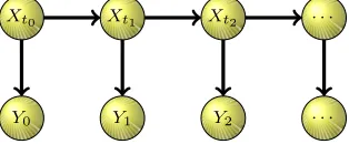The resulting recursive procedures for Fleming–Viot and Dawson–Watanabe signals that describe how to compute the parameters of the mixtures at each observation time are given in Propositions3.1and3.2, and the associated pseudo codes are outlined in Algorithms1 and2.

Fig 2_{. Hidden Markov model represented as a graphical model.}

1.2. Hidden Markov models

Since our time-dependent Bayesian nonparametric models are formulated as hidden Markov models, we introduce here some basic related notions. A hidden Markov model (HMM) is a double sequence {(Xtn, Yn), n ≥ 0} where Xtn is

an unobserved Markov chain, calledlatent signal, and Yn :=Ytn are

condition-ally independent observations given the signal. Figure 2 provides a graphical representation of an HMM. We will assume here that the signal is the discrete time sampling of a continuous time Markov process Xt with transition

ker-nel Pt(x,dx). The signal parametrises the law of the observations L(Yn|Xtn),

calledemission distribution. When this law admits density, this will be denoted byfx(y).

Filtering optimally an HMM requires the sequential exact evaluation of the so-called filtering distributions L(Xtn|Y0:n), i.e., the laws of the signal at

dif-ferent times given past and present observations, where Y0:n = (Y1, . . . , Yn).

Denoteνn :=L(Xtn|Y0:n) and letν be the prior distribution forXt0. The exact

or optimal filter is the solution of the recursion

ν0=φYt0(ν), νn=φYtn(ψtn−tn−1(νn−1)), n∈N. (1.2)

This involves the following two operators acting on measures: theupdate oper-ator, which in case a density exists takes the form

φy(ν)(dx) =

fx(y)ν(dx)

pν(y)

, pν(y) =

Xfx(y)ν(dx), (1.3)

and theprediction operator

ψt(ν)(dx) =

Xν(dx)Pt(x,dx

_{). (1.4)}

The update operation amounts to an application of Bayes’ Theorem to the currently available distribution conditional on the incoming data. The prediction operator propagates forward the current law of the signal of timetaccording to the transition kernel of the underlying continuous-time latent process. The above recursion (1.2) then alternates updates given the incoming data and predictions of the latent signal as follows:

L(Xt0)

update

−→ L(Xt0 |Y0)

prediction

−→ L(Xt1 |Y0)

update

−→ L(Xt1 |Y0, Y1)

IfXt0 has priorν=L(Xt0), thenν0=L(Xt0|Y0) is the posterior conditional on

the data observed at timet0; ν1 is the law of the signal at timet1 obtained by propagatingν0of at1−t0interval and conditioning on the dataY0, Y1observed at timet0andt1; and so on.

1.3. Illustration for CIR and WF signals

In order to appreciate the ideas behind the main theoretical results and the Algo-rithms we develop in this article, we provide some intuition on the corresponding results for one-dimensional hidden Markov models based on Cox–Ingersoll–Ross (CIR) and Wright–Fisher (WF) signals. These are the one-dimensional projec-tions of the DW and FV processes respectively, so informally we could say that a CIR process stands to a DW process as a gamma distribution stands to a gamma random measure, and a one-dimensional WF stands to a FV process as a Beta distribution stands to a Dirichlet process. The results illustrated in this section follow from Papaspiliopoulos and Ruggiero (2014) and are based on the interplay between computable filtering and duality of Markov processes, summarised later in Section4.1. The developments in this article rely on these results, which are extended to the infinite-dimensional case. Here we highlight the mechanisms underlying the explicit filters with the aid of figures, and post-pone the mathematical details to Section4.

First, let the signal be a one-dimensional Wright–Fisher diffusion on [0,1], with stationary distribution π = Beta(α, β) (see Section 2.1.2), which is also taken as the priorνfor the signal at time 0. The signal can be interpreted as the evolving frequency of type-1 individuals in a population of two types whose indi-viduals generate offspring of the same type of the parent, which may be subject to mutation. The observations are assumed to be Bernoulli with success prob-ability given by the signal state. Upon observation of yt0 = (yt0,1, . . . , yt0,m),

assuming it gives m1 type-1 and m2 type-2 individuals with m = m1+m2, the prior ν = π is updated as usual via Bayes’ theorem to ν0 = φyt0(ν) =

Beta(α+m1, β+m2). Here φy is the update operator (1.3). A forward propa-gation of these distribution of timetby means of the prediction operator (1.4) yields the finite mixture of Beta distributions

ψt(ν0) =

(0,0)≤(i,j)≤(m1,m2)

p(m1,m2),(i,j)(t)Beta(α+i, β+j),

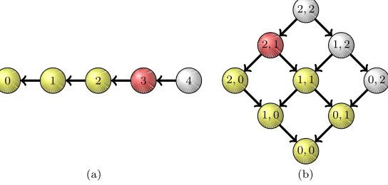
Fig 3_{. The death process on the lattice modulates the evolution of the mixture weights in the}

filtering distributions of models with CIR (left) and WF (right) signals. Nodes on the graph identify mixture components in the filtering distribution. The mixture weights are assigned according to the probability that the death process starting from the (red) node which encodes the current full information (herey= 3for the CIR and(m1, m2) = (2,1)for the WF) is in

a lower node after timet.

The time-varying mixing weights are the transition probabilities of an associated (dual) 2-dimensional death process, which can be thought of as jumping to lower nodes in the graph of Figure 3-(b) at a specified rate in continuous time. The effect on the mixture of these weights is that as time increases, the probability mass is shifted from components with parameters close to the full information (α+m1, β+m2), to components which bear less to none information on the data. The mass shift reflects the progressive obsolescence of the data collected at t0 as evaluated by signal law at timet0+t as tincreases, and in absence of further data the mixture converges to the prior/stationary distributionπ.

Note that it is not obvious that (1.4) yields a finite mixture whenPt is the

transition operator of a WF process, since Pt has an infinite series expansion

(see Section2.1.2). This has been proved rather directly in Chaleyat-Maurel and Genon-Catalot (2009) or by combining results on optimal filtering with some duality properties of this model (see Papaspiliopoulos and Ruggiero (2014) or Section 4here).

Consider now the model where the signal is a one-dimensional CIR diffusion on R+, with gamma stationary distribution (and prior at t0 = 0) given by

π = Ga(α, β) (see Section 2.2.2). The observations are Poisson with intensity given by the current state of the signal. If the first data are collected at time t1> t0, the forward propagation of the signal distribution to timet1 yields the same distribution by stationarity. Upon observation at timet1ofm≥1 Poisson data points with total count y, the priorν =πis updated via Bayes’ theorem to

ν0= Ga(α+y, β+m) (1.5)

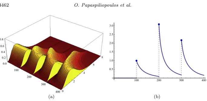
Fig 4_{. Temporal evolution of the filtering distribution (solid black in right panels and marginal}

rightmost section of left panels) under the CIR model: (a) until the first data collection the propagation preserves the prior/stationary distribution (red dotted in right panels); at the first data collection, the prior is updated to the posterior (blue dotted in right panels) via Bayes’ Theorem, determining a jump in the filtering process (left panel); (b) the forward propagation of the filtering distribution behaves as a finite mixture of Gamma densities (weighted compo-nents dashed coloured in right panel); (c) in absence of further data, the time-varying mixing weights shift mass towards the prior component, and the filtering distribution converges to the stationary law.

propagation ofν0 yields the finite mixture of gamma distributions

ψt(ν0) =

0≤i≤y

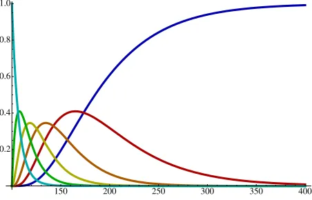
Fig 5_{. Evolution of the mixture weights which drive the mixture distribution in Fig.4. At} the jump time 100 (the origin here), the mixture component with full posterior information (blue dotted in Fig. 4) has weight equal to 1 (cyan curve), and the other components have zero weight. As the filtering distribution is propagated forward, the weights evolve as transi-tion probabilities of an associated death process. The mixture component equal to the prior distribution (red dotted in Fig.4), which carries no information on the data, has weight (blue curve) that is 0 at the jump time when the posterior update occurs, and eventually goes back to 1 in absence of further incoming observations, in turn determining the convergence of the mixture to the prior in Fig.4.

whose mixing weights also depend ont (see Lemma4.2below for their precise definition). At time t1+t, the filtering distribution is a (y+ 1)-components mixture with the first gamma parameter ranging from full (i=y) to null (i= 0) information with respect to the collected data (Figure 4-(b)). The time-dependent mixture weights are the transition probabilities of a certain associated (dual) one-dimensional death process, which can be thought of as jumping to lower nodes in the graph of Figure 3-(a) at a specified rate in continuous time. Similarly to the WF model, the mixing weights shift mass from components whose first parameter is close to the full information, i.e. (α+y, β+St), to

components which bear less to none information (α, β+St). The time evolution

of the mixing weights is depicted in Figure 5, where the cyan and blue lines are the weights of the components with full and no information on the data respectively. As a result of the impact of these weights on the mixture, the latter converges, in absence of further data, to the prior/stationary distribution π as t increases, as shown in Figure4-(c). Unlike the WF case, in this model there is a second parameter controlled by a deterministic (dual) process St on

R+ which subordinates the transitions of the death process; see Lemma 4.2. Roughly speaking, the death process on the graph controls the obsolescence of the observation countsy, whereas the deterministic processSt controls that of

the sample sizem. At the update timet1we haveS0=mas in (1.5), butStis a

deterministic, continuous and decreasing process, and in absence of further data Stconverges to 0 ast→ ∞, to restore the prior parameterβin the limit of (1.6).

Fig 6_{. Evolution of the filtering distribution (a) and of the deterministic component of the}

dual process (b) that modulates the sample size parameter in the mixture components, in the case of multiple data collection at time100,200,300.

When more data samples are collected at different times, the update and propagation operations are alternated, resulting in jump processes for both the filtering distribution and the deterministic dualSt(Figure6).

1.4. Preliminary notation

Although most of the notation is better introduced in the appropriate places, we collect here that which is used uniformly over the paper, to avoid recalling these objects several times throughout the text. In all subsequent sections, Y will denote a locally compact Polish space which represents the observations space,M(Y) is the associated space of finite Borel measures onY andM1(Y) its subspace of probability measures. A typical elementα∈M(Y) will be such that

α=θP0, θ >0, P0∈M1(Y), (1.7)

whereθ=α(Y) is the total mass of α, and P0 is sometimes called centering or baseline distribution. We will assume here thatP0 has no atoms. Furthermore, forαas above, Παwill denote the law onM1(Y) of a Dirichlet process, and Γβα

that onM(Y) of a gamma random measure, withβ >0. These will be recalled formally in Sections2.1.1and2.2.1.

We will denote by Xt the Fleming–Viot process and by Zt the Dawson–

Watanabe process, to be interpreted as{Xt, t≥0}and{Zt, t≥0}when written

without argument. Hence Xt and Zt take values in the space of continuous

functions from [0,∞) to M1(Y) andM(Y) respectively. We will write Xt(A)

and Zt(A) for their respective one dimensional projections onto the Borel set

x= (x1, . . . , xK)∈RK+, m= (m1, . . . , mK)∈ZK+, xm=xm1

1 · · ·x

mK

K , |x|=

K i=1xi,

where the dimension 2 ≤K ≤ ∞ will be clear from the context unless speci-fied. Accordingly, the Wright–Fisher model, closely related to projections of the Fleming–Viot process onto partitions, will be denoted Xt. We denote by0the

vector of zeros and by ei the vector whose only non zero entry is a 1 at the

ith coordinate. Let also “<” define a partial ordering on ZK+, so that m <n if mj ≤nj for all j ≥1 and mj < nj for some j ≥1. Finally, we will use the

compact notationy1:m for vectors of observationsy1, . . . , ym.

2. Hidden Markov measures

2.1. Fleming–Viot signals

2.1.1. The static model: Dirichlet processes and mixtures thereof

The Dirichlet process on a state space Y, introduced by Ferguson (1973) (see Ghosal (2010) for a recent review), is a discrete random probability measure x∈M1(Y). The process admits the series representation

x(·) =

∞

i=1

WiδYi(·), Wi=

Qi

j≥1Qj

, Yi iid

∼P0, (2.1)

where (Yi)i≥1 and (Wi)i≥1 are independent and (Qi)i≥1 are the jumps of a gamma process with mean measureθy−1e−ydy. We will denote by Πα the law

ofx(·) in (2.1), withαas in (1.7).

Mixtures of Dirichlet processes were introduced in Antoniak (1974). We say that xis a mixture of Dirichlet processes if

x|u∼Παu, u∼H,

where αu denotes the measureαconditionally onu, or equivalently

x∼

UΠαudH(u). (2.2)

With a slight abuse of terminology we will also refer to the right hand side of the last expression as a mixture of Dirichlet processes.

The Dirichlet process and mixtures thereof have two fundamental properties that are of great interest in statistical learning (Antoniak, 1974):

• Conjugacy: letxbe as in (2.2). Conditionally onmobservationsyi|x iid

∼x, we have

x|y1:m∼

UΠαu+

m

whereHy1:m is the conditional distribution ofugiveny1:m. Hence a

poste-rior mixture of Dirichlet processes is still a mixture of Dirichlet processes with updated parameters.

• Projection: letxbe as in (2.2). For any measurable partitionA1, . . . , AK

ofY, we have

(x(A1), . . . , x(AK))∼

UπαudH(u),

whereαu= (αu(A1), . . . , αu(AK)) andπαdenotes the Dirichlet

distribu-tion with parameter α.

Letting H be concentrated on a single point of U recovers the respective properties of the Dirichlet process as special case, i.e. x∼ Πα and yi|x

iid

∼ x imply respectively that x|y1:m ∼ Πα+m

i=1δyi and (x(A1), . . . , x(AK)) ∼ πα,

whereα= (α(A1), . . . , α(AK)).

2.1.2. The Fleming–Viot process

Fleming–Viot (FV) processes are a large family of diffusions taking values in the subspace ofM1(Y) given by purely atomic probability measures. Hence they describe evolving discrete distributions whose support also varies with time and whose frequencies are each a diffusion on [0,1]. Two states apart in time of a FV process are depicted in Figure7. See Ethier and Kurtz (1993) and Dawson (1993) for exhaustive reviews. Here we restrict the attention to a subclass known as the (labelled)infinitely many neutral alleles model with parent independent mutation, henceforth for simplicity called the FV process, which has the law of a Dirichlet process as stationary measure (Ethier and Kurtz,1993, Section 9.2). One of the most intuitive ways to understand a FV process is to consider its transition function, found in Ethier and Griffiths (1993). This is given by

Pt(x,dx) = ∞

m=0

dm(t)

Ym

Πα+m

i=1δyi(dx _)xm_(dy

1, . . . ,dym) (2.3)

where xm _{denotes the m-fold product measurex× · · · ×xand Π} α+m

i=1δyi is

a posterior Dirichlet process as defined in the previous section. The expression (2.3) has a nice interpretation from the Bayesian learning viewpoint. Given the current state of the processx, with probabilitydm(t) anm-sized sample fromxis

taken, and the arrival state is sampled from the posterior law Πα+m

i=1δyi. Here

dm(t) is the probability that anN-valued death process which starts at infinity at

time 0 is inmat timet, if it jumps frommtom−1 at rateλm=1₂m(θ+m−1).

See Tavar´e (1984) for details. Hence a largertimplies sampling a lower amount of information fromxwith higher probability, resulting in fewer atoms shared by xandx. The starting and arrival states thus have correlation which decreases intas controlled bydm(t). Ast→0, infinitely many samples are drawn fromx,

Fig 7. Two states of a FV process on[0,1]at successive times (solid discrete measures): (a) the initial state has distributionΠα0 withα0=θBeta(4,2)(dotted); (b) after some time, the

process reaches the stationary state, which has distributionΠαwithα=θBeta(2,4)(dashed).

the probabilities dm(t) in (2.3) is eventually absorbed in 0, which implies that

Pt(x,dx)→Παas t→ ∞, sox is sampled from the prior Πα. Therefore this

FV is stationary with respect to Πα (in fact, it is also reversible). It follows

that, using terms familiar to the Bayesian literature, under this parametrisa-tion the FV can be considered as a dependent Dirichlet process with continuous sample paths. Constructions of Fleming–Viot and closely related processes us-ing ideas from Bayesian nonparametrics have been proposed in Walker et al. (2007); Favaro et al. (2009); Ruggiero and Walker (2009a,b). Different classes of diffusive dependent Dirichlet processes or related constructions based on the stick-breaking representation (Sethuraman, 1994) are proposed in Mena and Ruggiero (2016); Mena et al. (2011).

Projecting a FV process Xt onto a measurable partition A1, . . . , AK of Y

yields a K-dimensional Wright–Fisher (WF) diffusion Xt, which is reversible

and stationary with respect to the Dirichlet distributionπα, forαi=θP0(Ai),

i= 1, . . . , K. See Dawson (2010); Etheridge (2009). This property is the dynamic counterpart of the projective property of Dirichlet processes discussed in Section 2.1.1. Consistently, the transition function of a WF process is obtained as a specialisation of the FV case, yielding

Pt(x,dx) = ∞

m=0

dm(t)

m∈ZK

+:|m|=m

m m

xmπα+m(dx) (2.4)

For statistical modelling it is useful to introduce a further parameterσthat controls the speed of the process. This can be done by defining the time change Xτ(t)withτ(t) =σt. In such parameterisation,σdoes not affect the stationary distribution of the process, and can be used to model the dependence structure.

2.2. Dawson–Watanabe signals

2.2.1. The static model: Gamma random measures and mixtures thereof

Gamma random measures (Lo,1982) can be thought of as the counterpart of Dirichlet processes in the context of finite intensity measures. A gamma random measure z ∈ M(Y) with shape parameter α as in (1.7) and rate parameter β >0, denotedz∼Γβ

α, admits representation

z(·) =β−1

∞

i=1

QiδYi(·), Yi iid

∼P0, (2.5)

with (Qi)i≥1 as in (2.1).

Similarly to the definition of mixtures of Dirichlet processes (Section2.1.1), we say thatzis a mixture of gamma random measures ifz∼_UΓβ_αudH(u), and with a slight abuse of terminology we will also refer to the right hand side of the last expression as a mixture of gamma random measures. Analogous conjugacy and projection properties to those seen for mixtures of Dirichlet processes hold for mixtures of gamma random measures:

• Conjugacy: letN be a Poisson point process onY with random intensity measurez, i.e., conditionally onz,N(Ai)

ind

∼ Po(z(Ai)) for any measurable

partition A1, . . . , AK of Y, K ∈ N. Let m := N(Y), and given m, let

y1, . . . , ymbe a realisation of points ofN, so that

yi|z, m iid

∼z/|z|, m|z∼Po(|z|) (2.6)

where |z|:=z(Y) is the total mass ofz. Then

z|y1:m∼

UΓ β+1

αu+m

i=1δyidHy1:m(u), (2.7)

whereHy1:mis the conditional distribution ofugiveny1:m. Hence mixtures

of gamma random measures are conjugate with respect to Poisson point process data.

• Projection: for any measurable partitionA1, . . . , AK ofY, we have

(z(A1), . . . , z(AK))∼

U K

i=1

Ga(αu,i, β)dH(u),

where αu,i=αu(Ai), and Ga(α, β) denotes the gamma distribution with

erties of gamma random measures as special case, i.e.z∼Γβ

αandyi as in (2.6)

implyz|y1:m∼Γβ_α+1₊m

i=1δyi, and the vector (z(A1), . . . , z(AK)) has independent

components z(Ai) with gamma distribution Ga(αi, β),αi=α(Ai).

Finally, it is well known that (2.1) and (2.5) satisfy the relation in distribution

x(·)=d z(·)

z(Y) (2.8)

where x is independent of z(Y). This extends to the infinite dimensional case the well known relationship between beta and gamma random variables. See for example Daley and Vere-Jones (2008), Example 9.1(e). See also Konno and Shiga (1988) for an extension of (2.8) to the dynamic case concerning FV and DW processes, which requires a random time change.

2.2.2. The Dawson–Watanabe process

Dawson–Watanabe (DW) processes can be considered as dependent models for gamma random measures, and are, roughly speaking, the gamma counterpart of FV processes. More formally, they are branching measure-valued diffusions taking values in the space of finite discrete measures. As in the FV case, they describe evolving discrete measures whose support varies with time and whose masses are each a positive diffusion, but relaxing the constraint of their masses summing to one to that of summing to a finite quantity. See Dawson (1993) and Li (2011) for reviews. Here we are interested in the special case of subcritical branching with immigration, where subcriticality refers to the fact that in the underlying branching population, which can be used to construct the process, the mean number of offspring per individual is less than one. Specifically, we will consider DW processes with transition function

Pt(z,dz) = ∞

m=0

d|z|,β_m (t)

Ym

Γβ+S∗t α+m

i=1δyi(dz

_)(z/|z|)m_(dy

1, . . . ,dym). (2.9)

where

d|_mz|,β(t) = Po

m |z|β eβt/2₋₁

and S_t∗:= β eβt/2₋₁.

See Ethier and Griffiths (1993b). The interpretation of (2.9) is similar to that of (2.3): conditional on the current state given by the measurez,miid samples are drawn from the normalised measurez/|z|and the arrival statezis sampled from Γβ+St∗

α+m

i=1δyi. Here the main structural difference with respect to (2.3),

apart from the different distributions involved, is that since in general St∗ is

not an integer quantity, the interpretation as sampling the arrival statez from a posterior gamma law is not formally correct; cf. (2.7). The sample size m is chosen with probability d|z|,βm (t), which is the probability that an N-valued

frommtom−1 at rate (mβ/2)(1−eβt/2₎−1_{. See Ethier and Griffiths (1993b)} for details. So z and z will share fewer atoms the farther they are apart in time. The DW process with the above transition is known to be stationary and reversible with respect to the law Γβ

α of a gamma random measure; cf. (2.5).

See Shiga (1990); Ethier and Griffiths (1993b). The Dawson–Watanabe process has been recently considered as a basis to build time-dependent gamma process priors with Markovian evolution in Caron and Teh (2012) and Span`o and Lijoi (2016).

The DW process satisfies a projective property similar to that seen in Sec-tion2.1.2for the FV process. Let Zthave transition (2.9). Given a measurable

partition A1, . . . , AK of Y, the vector (Zt(A1), . . . , Zt(AK)) has independent

components zt,i = Zt(Ai) each driven by a Cox–Ingersoll–Ross (CIR)

diffu-sion (Cox et al., 1985). These are also subcritical continuous-state branching processes with immigration, reversible and ergodic with respect to a Ga(αi, β)

distribution, with transition function

Pt(zi,dzi) = ∞

mi=0 Po

mi

ziβ

eβt/2₋₁

Ga

dz αi+mi, β+St∗

. (2.10)

As for FV and WF processes, a further parameterσthat controls the speed of the process can be introduced without affecting the stationary distribution. This can be done by defining an appropriate time change that can be used to model the dependence structure.

3. Conjugacy properties of time-evolving Dirichlet and gamma random measures

3.1. Filtering Fleming–Viot signals

Let the latent signal Xt be a FV process with transition function (2.3). We

assume that, given the signal state, observations are drawn independently from x, i.e. as in (1.1) with Xt = x. Since x is almost surely discrete (Blackwell,

1973), a sample y1:m = (y1, . . . , ym) from xwill feature Km ≤ m ties among

the observations with positive probability. Denote by (y₁∗, . . . , y_Km∗ ) the distinct values iny1:mand bym= (m1, . . . , mKm) the associated multiplicities, so that

|m|=m. When an additional sampleym+1:m+n with multiplicitiesnbecomes

available, we adopt the convention that nadds up to the multiplicities of the types already recorded iny1:m, so that the total multiplicities count is

m+n= (m1+n1, . . . , mKm+nKm, nKm+1, . . . , nKm+n). (3.1)

The following Lemma states in our notation the special case of the conjugacy for mixtures of Dirichlet processes which is of interest here; see Section 2.1.1. To this end, let

Section 1.4. Denote also by PUα(ym+1:m+n | y1:m) the joint distribution of

ym+1:m+n giveny1:mwhen the random measurexis marginalised out, which is

determined by the Blackwell–MacQueen P´olya urn predictive scheme (Blackwell and MacQueen, 1973)

Ym+i+1|y1:m+i∼

θP0+ m+i

j=1 δyj

θ+m+i , i= 0, . . . , n−1.

Lemma 3.1. Let M ⊂ M, α as in (1.7) and x be the mixture of Dirichlet processes

x∼

m∈M

wmΠ_α+Km i=1miδy∗_i,

with_m∈Mwm= 1. Given an additionaln-sized sampleym+1:m+n fromxwith

multiplicitiesn, the update operator (1.3)yields

φym+1:m+n

m∈M

wmΠ_α+Km i=1miδy_i∗

=

m∈M

ˆ

wmΠ_α+Km+n

i=1 (mi+ni)δy_i∗

, (3.3)

where

ˆ

wm∝wmPUα(ym+1:m+n|y1:m). (3.4)

Here “∝” denotes proportionality. The updated distribution is thus still a mixture of Dirichlet processes with different multiplicities and possibly new atoms in the parameter measuresα+Km+n

i=1 (mi+ni)δyi∗.

The following Theorem formalises our main result on FV processes, showing that the family of finite mixtures of Dirichlet processes is conjugate with respect to discretely sampled data as in (1.1) withXt=x. ForMas in (3.2), let

L(m) ={n∈ M: 0≤n≤m}, m∈ M,

L(M) ={n∈ M: 0≤n≤m,m∈M}, M ⊂ M, (3.5)

be the set of nonnegative vectors lower than or equal to m or to those in M respectively, with “≤” defined as in Section (1.4). For example, in Figure3,L(3) andL((1,2)) are both given by all yellow and red nodes in each case. Let also

p(i;m,|i|) =

|m| |i|

−1

j≥1

mj

ij

(3.6)

be the multivariate hypergeometric probability function, with parameters (m,|i|), evaluated ati.

Theorem 3.1. Letψtbe the prediction operator(1.4)associated to a FV process

with transition operator (2.3). Then the prediction operator yields as t -time-ahead propagation the finite mixture of Dirichlet processes

ψt

Π_α+Km i=1miδy∗_i

=

n∈L(m)

pm,n(t)Π_α+Km

withL(m)as in (3.5) and where

pm,m−i(t) =

e−λ|m|t_{, i=0}

C_|m|,|m|−|i|(t)p(i;m,|i|), 0<i≤m,

(3.8)

with

C_|m|,|m|−|i|(t) =

|i|−1

h=0

λ_|m|−h

(−1)|i|

|i|

k=0

e−λ|m|−kt

0≤h≤|i|,h=k(λ|m|−k−λ|m|−h)

,

λn=n(θ+n−1)/2 andp(i;m,|i|) as in (3.6).

The transition operator of the FV process thus maps a Dirichlet process at time t0 into a finite mixture of Dirichlet processes at time t0+t. The mixing weights are the transition probabilities of a death process on the Km

dimen-sional lattice, withKmbeing as in (3.7) the number of distinct values observed

in previous data. The result is obtained by means of the argument described in Figure1, which is based on the property that the operations of propagating and projecting the signal commute. By projecting the current distribution of the signal onto an arbitrary measurable partition, yielding a mixture of Dirich-let distributions, we can exploit the results for finite dimensional WF signals to yield the associated propagation (Papaspiliopoulos and Ruggiero,2014). The propagation of the original signal is then obtained by means of the character-isation of mixtures of Dirichlet processes via their projections. See Section4.2 for a proof. In particular, the result shows that under these assumptions, the prediction operation (1.4) with the transition function (2.3) reduces to a finite sum.

Iterating the update and propagation operations provided by Lemma3.1and Theorem3.1allows to perform sequential Bayesian inference on a hidden signal of FV type by means of a finite computation. Here the finiteness refers to the fact that the infinite dimensionality due to the transition function of the signal is avoided analytically, without resorting to any stochastic truncation method for (2.3), given, e.g., by Walker (2007); Papaspiliopoulos and Roberts (2008), and the computation can be conducted in closed form.

The following Proposition formalises the recursive algorithm that sequentially evaluates the marginal posterior laws L(Xtn|Y1:n) of a partially observed FV

process by alternating the update and propagation operations, and identifies the family of distributions which is closed with respect to these operations. Define the family of finite mixtures of Dirichlet processes

FΠ=

m∈M

wmΠα+Km_i=1miδy∗_i :M ⊂ M,|M|<∞, wm≥0,

m∈M

wm= 1

,

withMas in (3.2) and for a fixedαas in (1.7). Define also

t(y,m) =m+n, m∈ZK₊ so thatt(y,m) is (3.1) ifnare the multiplicities ofy, and

invariant law Πα defined as in Section 2.1.1, and suppose data are collected as

in (1.1) with Xt = x. Then FΠ is closed under the application of the update

and prediction operators (1.3)and (1.4). Specifically,

φym+1:m+n

m∈M

wmΠ_α+Km i=1miδy∗_i

=

n∈t(ym+1:m+n,M)

ˆ

wnΠ_α+Km+n i=1 niδy∗_i

,

(3.10)

with t(y, M)as in (3.9),

ˆ

wn∝wmPUα(ym+1:m+n |y1:m) for n=t(y,m),

n∈t(y,M) wn= 1,

and

ψt

m∈M

wmΠ_α+Km i=1miδy_i∗

=

n∈L(M)

p(M,n, t)Π_α+Km

i=1niδy∗_i, (3.11)

with

p(M,n, t) = m∈M,m≥n

wmpm,n(t) (3.12)

andpm,n(t)as in (3.8).

Note that the update operation (3.10) preserves the number of components in the mixture, while the prediction operation (3.7) increases its number. The intu-ition behind this point is analogous to the illustration in Section1.3, where the prior (node (0,0)) is updated to the posterior (node (2,1)) and propagated into a mixture (coloured nodes), with the obvious difference that here the maximum number of distinct values is unbounded and not fixed.

Algorithm1describes in pseudo-code the implementation of the filter for FV processes.

3.2. Filtering Dawson–Watanabe signals

Let now the signalZtfollow a DW process with transition function (2.9), with

invariant measure given by the law Γβαof a gamma random measure; see (2.5).

We assume that, given the signal state, observations are drawn from a Poisson point process with intensityz, i.e., as in (2.6) withZt=z. Analogously to the

FV case, since z is almost surely discrete, a sample y1:m = (y1, . . . , ym) from

(2.6) will featureKm≤mties among the observations with positive probability.

To this end, we adopt the same notation as in Section3.1.

Algorithm 1:Filtering algorithm for FV signals

Data:yt_j = (ytj,1, . . . , ytj,mtj) at timestj,j= 0, . . . , J, as in (1.1)

Set prior parametersα=θP0,θ >0,P0∈M1(Y)

Initialise

y← ∅,y∗=∅,m←0,m←0,M← {0},Km←0,w0←1

Forj= 0, . . . , J

Compute data summaries

read dataytj

m←m+ card(ytj)

y∗←distinct values iny∗∩yt_j

Km←card(y∗) Update operation

for m∈M

n←t(yt_j,m)

wn←wmPUα(ytj |y)

M←t(yt_j, M)

for m∈M

wm←wm/∈Mw

Xtj |y,ytj ∼

m∈MwmΠα+Km_i=1miδ_y∗

i Propagation operation

for n∈L(M)

wn←p(M,n, tj+1−tj) as in (3.12)

M←L(M) Xtj+1|y,ytj ∼

m∈MwmΠα+Km_i=1miδy∗_i y←y∪ytj

Lemma 3.2. LetMbe as in(3.2),M ⊂ M,αas in (1.7)andzbe the mixture of gamma random measures

z∼

m∈M

wmΓβ_α+1₊Km i=1miδy∗_i

,

with _m∈Mwm = 1. Given an additional n-sized sampleym+1:m+n from z as

in (2.6) with multiplicitiesn, the update operator (1.3)yields

φym:m+n

m∈M

wmΓβ_α+1₊Km i=1miδy∗_i

=

m∈M

ˆ wmΓβ+2

α+Km_i=1+n(mi+ni)δy∗_i

, (3.13)

withwˆm as in (3.4).

The updated distribution is thus still a mixture of gamma random measures with updated parameters and the same number of components.

cess with transition operator (2.9). Let alsoL(M)be as in (3.5). Then the pre-diction operator yields ast-time-ahead propagation the finite mixture of gamma random measures

ψt

Γβ+s

α+Km_i=1miδy∗_i

=

n∈L(m) ˜

pm,n(t)Γβ_α+₊StKm i=1niδy_i∗

, (3.14)

where

˜

pm,n(t) = Bin(|m| − |n|;|m|, p(t))p(n; m,|n|), (3.15)

and

p(t) =St/S0, St=

βS0 (β+S0)eβt/2−S0

, S0=s. (3.16)

with p(n;m,|n|)as in (3.6) andBin(|m| − |n|;|m|, p(t))denoting a Binomial pmf with parameters (|m|, p(t))evaluated at|m| − |n|.

The transition operator of the DW process thus maps a gamma random mea-sure into a finite mixture of gamma random meamea-sures. The time-varying mixing weights factorise into the binomial transition probabilities of a one-dimensional death process starting at the total size of previous data|m|and into a hyperge-ometric pmf. The intuition is that the death process regulates how many levels down theKm dimensional lattice are taken, and the hypergeometric

probabil-ity chooses which admissible path down the graph is chosen given the arrival level. In Figure 3 we would have Km = 2 distinct values with multiplicites

m = (2,1) and total size |m| = 3. Then, e.g., ˜p(2,1),(1,1)(t), is given by the probability Bin(1; 3, p(t)) that the death process jumps down one level from 3 in timet (Figure3-(a)), times the probability p((1,1); (2,1),2), conditional on going down one level, of reaching (1,1) from (2,1) instead of (2,0), i.e. of re-moving one item from the pair and not the singleton observation. The Binomial transition of the one-dimensional death process is subordinated to a determinis-tic process Stwhich modulates the sample size continuously in (3.14), starts at

the valueS0=s(cf. the left hand side of (3.14)) and converges to 0 ast→ ∞. The result is obtained by means of a similar argument to that used for The-orem (3.1), jointly with the relation (2.8) (which here suffices to be applied at the margin of the process). In particular, we exploit the fact that the projec-tion of a DW process onto an arbitrary partiprojec-tion of the space yields a vector of independent CIR processes. See Section 4.3for a proof. Analogously to the FV case, the result shows that under the present assumptions, the prediction operation (1.4) with the transition function (2.9) reduces to a finite sum.

The following Proposition formalises the recursive algorithm that evaluates the marginal posterior laws L(Xtn|Y1:n) of a partially observed DW process,

allowing to perform sequential Bayesian inference on a hidden signal of DW type by means of a finite computation and within the family of finite mixtures of gamma random measures. Define such family as

FΓ=

m∈M

wmΓβ_α+₊sKm i=1miδy∗_i

s >0, M ⊂ M, |M|<∞, wm≥0,

m∈M

wm= 1

,

withMas in (3.2).

Proposition 3.2. Let Zt be a DW process with transition function (2.9) and

invariant law Γβ

α defined as in Section 2.2.1, and suppose data are collected as

in (2.6)withZt=z. ThenFΓ is closed under the application of the update and

prediction operators (1.3) and (1.4). Specifically,

φym+1:m+n

m∈M

wmΓβ_α+₊sKm i=1miδy_i∗

=

n∈t(ym+1:m+n,M)

ˆ

wnΓβ+s+1

α+Km_i=1+nniδy∗_i

,

(3.17)

witht(y, M)as in (3.9),wˆnas in Proposition3.1, and

ψt

m∈M

wmΓβ+s

α+Kmi=1miδy∗_i

=

n∈L(M)

p(M,n, t)Γβ+St

α+Kmi=1niδy∗_i

. (3.18)

with

p(M,n, t) = m∈M,m≥n

wmp˜m,n(t) (3.19)

andp˜m,n(t)as in (3.15)andSt as in (3.16).

Algorithm2describes in pseudo-code the implementation of the filter for DW processes.

4. Theory for computable filtering of FV and DW signals

4.1. Computable filtering and duality

A filter is said to be computable if the sequence of filtering distributions (the marginal laws of the signal given past and current data) can be characterised by a set of parameters whose computation is achieved at a cost that grows at most polynomially with the number of observations. See, e.g., Chaleyat-Maurel and Genon-Catalot (2006). Special cases of this framework are finite dimensional filters for which the computational cost is linear in the number of observations, the Kalman filter for linear Gaussian HMMs being the reference model in this setting.

Let X denote the state space of the HMM. Papaspiliopoulos and Ruggiero (2014) showed that the existence of a computable filter can be established if the following structures are embedded in the model:

Conjugacy: there exists a functionh(x,m, θ)≥0, where x∈ X,m ∈ZK

+ for some K ∈ N, and θ ∈ Rl _{for some l ∈ N, and functions t}

1(y,m) and

t2(y, θ) such that

h(x,m, θ)π(dx) = 1, for allm andθ, and

Algorithm 2: Filtering algorithm for DW signals

Data: (mtj,ytj) = (mtj, ytj,1, . . . , ytj,mtj) at timestj,j= 0, . . . , J, as in (2.6)

Set prior parametersα=θP0,θ >0,P0∈M1(Y),β >0

Initialise

y← ∅,y∗=∅,m←0,m←0,M← {0},Km←0,w0←1,s= 0

Forj= 0, . . . , J

Compute data summaries

read dataytj

m←m+ card(ytj)

y∗←distinct values iny∗∩yt_j

Km←card(y∗) Update operation

for m∈M

n←t(yt_j,m)

wn←wmPUα(ytj |y)

M←t(yt_j, M)

for m∈M

wm←wm/∈Mw

Xtj |y,ytj ∼

m∈MwmΓ β+s

α+Km_i=1miδy∗_i Propagation operation

for n∈L(M)

wn←p(M,n, tj+1−tj) as in (3.19)

M←L(M)

s←Stj+1−tj as in (3.16),S0=s

Xtj+1|y,ytj ∼

m∈MwmΓ β+s

α+Km_i=1miδy∗_i

s←s

y←y∪ytj

Hereh(x,m, θ)π(dx) identifies a parametric family of distributions which is closed under Bayesian updating with respect to the observation model. Two types of parameters are considered, a multi-indexmand a vector of real-valued parametersθ. The update operatorφy maps the distribution

h(x,m, θ)π(dx), conditional on the new observation y, into a density of the same family with updated parameterst1(y,m) andt2(y, θ). Typically

π(dx) is the prior andh(x,m, θ) is the Radon–Nikodym derivative of the posterior with respect to the prior, when the model is dominated. See, e.g., (4.6) below for an example of suchhwhenπis the Dirichlet distibution.

Duality: there exists a two-component Markov process (Mt,Θt) with

state-spaceZK

+×Rl and infinitesimal generator

(Ag)(m, θ) =λ(|m|)ρ(θ)

K

i=1

mi[g(m−ei, θ)−g(m, θ)]+ l

i=1

ri(θ)

∂g(m, θ) ∂θ

to the functionh, i.e., it satisfies

Ex_[h(X

t,m, θ)] =E(m,θ)[h(x, Mt,Θt)], (4.1)

for all x∈ X,m∈ZK

+, θ∈Rl, t≥0. Here Mt is a death process onZK+, i.e. a non-increasing pure-jump continuous time Markov process, which jumps frommtom−ei at rateλ(|m|)miρ(θ) and is eventually absorbed

at the origin; Θtis a deterministic process assumed to evolve autonomously

according to a system of ordinary differential equationsr(Θt) =dΘt/dtfor

some initial condition Θ0=θ0and a suitable functionr:Rl→Rl, whose

ith coordinate is denoted byri in the generatorA above and modulates

the death rates of Mt through ρ(θ). The expectations on the left and

right hand sides are taken with respect to the law of Xt and (Mt,Θt)

respectively, conditional on the respective starting points.

The duality condition (4.1) hides a specific distributional relationship be-tween the signal process Xt, which can be thought of as the forward process,

and the dual process (Mt,Θt), which can be thought of as unveiling some

fea-tures of the time reversal structure ofXt. Informally, the death process can be

considered as the time reversal of collecting data points if they come at random times, and the deterministic process, in the CIR example (see Section1.3), can be considered as a continuous reversal of the sample size process, which instead increases by steps. For example, in the well known duality relation between the WF diffusion and the block counting process of Kingman’s coalescent, the lat-ter describes the number of surviving non mutant lines of descent in the tree backwards in time which tracks the ancestors of a sample of individuals in the current population. See Griffiths and Span`o (2010). See also Jansen and Kurt (2014) for a review of duality structures for Markov processes.

Note that a local sufficient condition for (4.1), usually easier to check, is

(Ah(·,m, θ))(x) = (Ah(x,·,·))(m, θ), (4.2)

for all ∀x ∈ X,m ∈ Z+K, θ ∈ Rl, where A is as above and A denotes the infinitesimal generator of the signalXt.

Under the above conditions, Proposition 2.3 of Papaspiliopoulos and Ruggiero (2014) shows that given the family of distributions

F=

h(x,m, θ)π(dx),m∈ZK₊, θ∈Rl

,

ifν∈ F, then the filtering distributionνnwhich satisfies (1.2) is a finite mixture

of distributions inFwith parameters that can be computed recursively. This in turn implies that the family of finite mixtures of elements ofF is closed under the iteration of update and prediction operations.

The interpretation is along the lines of the illustration of Section 1.3. Here π, the stationary measure of the forward process, plays the role of the prior distribution and is represented by the origin ofZK