warwick.ac.uk/lib-publications
Original citation:
Veras, Dimitri, Mustill, Alexander J., Gaensicke, B. T., Redfield, Seth, Georgakarakos,
Nikolaos, Bowler, Alex B. and Lloyd, Maximillian J. S.. (2016) Full-lifetime simulations of
multiple unequal-mass planets across all phases of stellar evolution. Monthly Notices of the
Royal Astronomical Society, 458 (4). pp. 3942-3967.
Permanent WRAP URL:
http://wrap.warwick.ac.uk/78569
Copyright and reuse:
The Warwick Research Archive Portal (WRAP) makes this work by researchers of the
University of Warwick available open access under the following conditions. Copyright ©
and all moral rights to the version of the paper presented here belong to the individual
author(s) and/or other copyright owners. To the extent reasonable and practicable the
material made available in WRAP has been checked for eligibility before being made
available.
Copies of full items can be used for personal research or study, educational, or not-for profit
purposes without prior permission or charge. Provided that the authors, title and full
bibliographic details are credited, a hyperlink and/or URL is given for the original metadata
page and the content is not changed in any way.
Publisher’s statement:
This article has been accepted for publication in Monthly Notices of the Royal Astronomical
Society © 2016 The Authors Published by Oxford University Press on behalf of the Royal
Astronomical Society. All rights reserved.
Link to final published version:
http://dx.doi.org/10.1093/mnras/stw476
A note on versions:
The version presented in WRAP is the published version or, version of record, and may be
cited as it appears here.
Full-lifetime simulations of multiple unequal-mass planets across all
phases of stellar evolution
Dimitri Veras,
1‹Alexander J. Mustill,
2Boris T. G¨ansicke,
1Seth Redfield,
3Nikolaos Georgakarakos,
4Alex B. Bowler
1and Maximillian J. S. Lloyd
11Department of Physics, University of Warwick, Coventry CV4 7AL, UK
2Lund Observatory, Department of Astronomy and Theoretical Physics, Lund University, Box 43, SE-221 00 Lund, Sweden 3Astronomy Department and Van Vleck Observatory, Wesleyan University, Middletown, CT 06459-0123, USA
4New York University Abu Dhabi, Saadiyat Island, PO Box 129188 Abu Dhabi, UAE
Accepted 2016 February 25. Received 2016 February 25; in original form 2016 January 27
A B S T R A C T
We know that planetary systems are just as common around white dwarfs as around main-sequence stars. However, self-consistently linking a planetary system across these two phases of stellar evolution through the violent giant branch poses computational challenges, and previous studies restricted architectures to equal-mass planets. Here, we remove this constraint and perform over 450 numerical integrations over a Hubble time (14 Gyr) of packed planetary systems with unequal-mass planets. We characterize the resulting trends as a function of planet order and mass. We find that intrusive radial incursions in the vicinity of the white dwarf become less likely as the dispersion amongst planet masses increases. The orbital meandering which may sustain a sufficiently dynamic environment around a white dwarf to explain observations is more dependent on the presence of terrestrial-mass planets than any variation in planetary mass. Triggering unpacking or instability during the white dwarf phase is comparably easy for systems of unequal-mass planets and systems of equal-mass planets; instabilities during the giant branch phase remain rare and require fine-tuning of initial conditions. We list the key dynamical features of each simulation individually as a potential guide for upcoming discoveries.
Key words: methods: numerical – celestial mechanics – minor planets, asteroids: general – planets and satellites: dynamical evolution and stability – protoplanetary discs – white dwarfs.
1 I N T R O D U C T I O N
Nearly 100 planets are known to orbit giant stars,1and signatures
of planetary systems have been detected at over 1000 white dwarfs (WDs). This latter number is obtained through observed plane-tary debris in WD atmospheres (Zuckerman et al.2003; Dufour et al.2007; Zuckerman et al.2010; Kleinman et al.2013; Koester, G¨ansicke & Farihi2014; Gentile Fusillo, G¨ansicke & Greiss2015; Kepler et al.2015,2016). About 40 of these WDs contain compact (≈0.6–1.2 R) planetary debris discs (see Farihi2016for a review), and one hosts at least six transiting planetesimals (WD 1145+017; Vanderburg et al.2015; Croll et al.2016; G¨ansicke et al. 2016; Rappaport et al.2016; Xu et al.2016). Also, planets around two other WDs have been observed (WD 0806−661 b; Luhman, Bur-gasser & Bochanski2011and PSR B1620−26AB b; Sigurdsson
E-mail:[email protected]
1www.lsw.uni-heidelberg.de/users/sreffert/giantplanets.html
et al.2003). Although the architectures of most WD planetary sys-tems remain unknown, these statistics demonstrate that the study of post-main-sequence planetary systems has entered a new era, one where we can begin to investigate population-wide trends as well as key individual systems.N-body simulations of multiplanet sys-tems represent a vital probe into their history and future, revealing insights about their formation and fate.
However, accurately performing multibody simulations across different phases of stellar evolution remains challenging. For bod-ies much smaller than planets, including gravity alone is likely to be insufficient (see fig. 2 of Veras2016). Asteroids within about 7 au of a main-sequence star could be spun up to fission during the giant branch (GB) phase of stellar evolution (Veras, Jacob-son & G¨ansicke2014c) due to intense radiation. Asteroids further away could have their orbits changed due to another radiation-based effect: the Yarkovsky drift (Veras, Eggl & G¨ansicke2015a). Fur-ther, the stellar wind could induce drag on asteroids and pebbles (Dong et al.2010; Veras et al.2015a), and sublimation of volatile substances on these objects could change their orbits (Veras, Eggl
C
2016 The Authors
& G¨ansicke 2015b) and/or launch ejecta, as speculated in WD 1145+017 (Vanderburg et al. 2015; Croll et al.2016; G¨ansicke et al.2016; Rappaport et al.2016; Xu et al.2016).
Even restricting simulations to planets presents challenges. (i) Tidal effects between planets and their parent stars can destroy or alter the planets, but just how remains an open question (see section 5 of Veras2016for a review). GB stars harbour radii that extend to several au, and planets too close to their parent stars may hence be engulfed on both the red giant branch (RGB) phase (e.g. Villaver et al.2014) and the asymptotic giant branch (AGB) phase (Mustill & Villaver2012). Nevertheless, only about half of the currently known exoplanets will likely be engulfed (Nordhaus & Spiegel2013), and observational biases against finding planets at large separations imply that the actual fraction is much less. (ii) Computational limitations hinder explorations with long main-sequence lifetimes or planets on close-in orbits. Only recently (Veras & G¨ansicke2015) have 14 Gyr (the current age of the Universe) simulations with main-sequence progenitor masses under 3 M (most WD progenitors had masses between about 1.5 and 2.5 M; Koester et al.2014) been carried out for ensembles of multiplanet systems,2as previous attempts (Duncan & Lissauer1998; Debes
& Sigurdsson2002; Veras et al.2013a; Mustill, Veras & Villaver 2014) did not achieve this coverage.
Nevertheless, up until now full-lifetime simulations of multi-planet systems have been restricted to equal-mass multi-planets. Although this assumption significantly helps constrain the available param-eter space to explore, real systems exhibit a variance of planetary masses of a few per cent to many orders of magnitude. Further, pre-vious studies have predominately modelled Jupiter-mass planets, which are rarer than terrestrial planets (Cassan et al.2012; Winn & Fabrycky2015). Further, no published study has simulated multiple planets with test particles.
Here, we break these barriers, and perform a suite of 14 Gyr simulations of unequal-mass planets, occasionally including test particles, in order to explore the consequences and resulting trends. In Section 2, we describe our setup. Section 3 details the classifica-tion scheme for our results, and the results themselves. We discuss the implications in Section 4, and conclude in Section 5.
Appendix A is our simulation data base. Each row of each table corresponds to one simulation, and within each row we present the salient dynamical features.
2 S I M U L AT I O N S E T U P
Simulations of planetary systems through multiple stages of stel-lar evolution require both the star and planets to be treated self-consistently as a function of time.
2.1 Numerical codes
Here, we have used an updated version of the code from Veras et al. (2013a), Mustill et al. (2014), Veras, Shannon & G¨ansicke (2014d) and Veras & G¨ansicke (2015), which combines planetary and stellar evolution. The stellar evolution is computed fromSSE(Hurley, Pols
& Tout 2000), which is more than sufficiently accurate for our purposes. If we instead desired to trace more detailed characteristics of a particular star, like its chemical profile, then perhaps a code
2A few individual planetary systems, or putative planetary systems, have
been modelled with simulations spanning multiple phases of evolution: HU Aqr (Portegies Zwart2013) and NN Ser (Mustill et al.2013).
like the increasingly utilizedMESA(Paxton et al.2011,2015) would be more suitable. However, here we need only the mass and radius evolution of the star, and did not model any particular known system; we ignored radiative effects, which are negligible for the types of planets we simulated.
The output fromSSEwas ported directly into a heavily modified
version of theMERCURYplanetary evolution code, originally from
Chambers (1999). Our version ofMERCURYused the Bulirsch–Stoer integrator throughout the simulation, ensuring accurate treatment of potential close encounters. We adopted a tolerance value of 10−13. Stellar mass and radius changes were interpolated within
each Bulirsch–Stoer timestep, helping to ensure accuracy. Stars which engulfed planets throughout the course of the simulations had masses which were increased accordingly. Our output frequency was 1 Myr; a shorter frequency would have prohibitively slowed down our simulations. As is theMERCURYdefault, any collisions
be-tween planets were treated as purely inelastic. Further, our modified code allowed for the tracking of the minimum orbital pericentre of all surviving planets, and adopted a standard Hill ellipsoid for the solar neighbourhood (Veras & Evans2013; Veras et al.2014a) to accurately track ejections.
2.2 Stellar properties
The enormous parameter space of our computationally demanding simulations forced us to adopt a single type of star for our simu-lations. Our star contained a physically motivated stellar mass of 2.0 Mon the main sequence. The present-day population of WDs, with average masses ranging from about 0.60 to 0.65 M(Liebert, Bergeron & Holberg 2005; Falcon et al.2010; Tremblay et al. 2013) corresponds to main-sequence A- and F-star progenitors (see fig. 3 of Veras2016), from which 2.0 Mis an appropriate value from the initial-to-final mass relation (Catal´an et al.2008; Kalirai et al.2008; Casewell et al.2009; Koester et al.2014). This value coincidentally also marks (i) the point beyond which the planet occurrence rate falls off (Reffert et al.2015) and (ii) a transition in evolutionary sequence due to stellar mass; below 2.0 Ma star would continue ascending the RGB until it undergoes a core helium flash, which changes the amount of mass lost and radius along the RGB. Lower mass stars have larger radii and greater mass-loss. Regardless, the greatest mass-loss (by several orders of magnitude) and radius changes occur along the AGB even for values within a few 0.1 of 2.0 M.
The evolution of the star is illustrated in Fig.1, characterized in Table1and described in this paragraph. Our 2.0 Mstar was as-sumed to have solar metallicity, and remained on the main sequence for 1.1735 Gyr. Along the RGB, the star lost mass according to the traditional3Reimers mass-loss prescription, with a numerical
co-efficient of 0.5. The star stayed on the RGB for 23 Myr and lost 0.002 Mduring that time, while expanding its radius out to 0.13 au. Afterwards, the star contracted to a radius of 0.04 au. The AGB phase began at 1.4894 Gyr, and lasted for only 6.4 Myr. However, during this time, the star lost 1.338 Mand expanded its radius out to 1.82 au; see Fig.1. Finally, the star ended its evolution as a WD formed with a mass of 0.6365 Mand a radius of 5×10⁻⁵au.
Varying the stellar mass within the code is nearly equivalent to assuming that the star loses mass isotropically. This assumption
3Schr¨oder & Cuntz (2005) provided an improved, physically motivated
Figure 1. The mass (left-hand panel) and radius (right-hand panel) evolution of the star used in this study, during the tip of the AGB phase and when the WD is born (at the start of the EWD=‘early white dwarf’ phase). Marked on the right-hand panel is the maximum AGB radius (Rmax) and the WD Roche radius (distance) adopted in this study (Rroche).
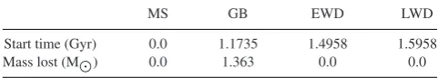
Table 1. Time at the beginning of each phase (MS =main sequence, GB=giant branch, EWD=early white dwarf, LWD=late white dwarf) and the total mass lost during those phases. The LWD phase lasts until the end of the simulations (14 Gyr).
MS GB EWD LWD
Start time (Gyr) 0.0 1.1735 1.4958 1.5958
Mass lost (M) 0.0 1.363 0.0 0.0
is excellent for orbiting bodies within a few hundred astronomical units (Veras, Hadjidemetriou & Tout2013b). Because the planets are assumed to be point masses, they do not accrete any of the stellar mass and the isotropic assumption is maintained; see sec-tion 4 of Veras (2016) for more details. This type of stellar mass decrease, however, does not consider the lag time between the ejecta passing beyond two different orbits. However, this effect should be negligible; see section 2 of Payne et al. (2016) for quantification.
A planet that ventures into the vicinity of the WD might be dis-rupted or destroyed. This ‘vicinity’ may extend to a few hundred times the WD radius. The critical radius at which disruption occurs (known as the Roche radius), however, is dependent on the planet’s shape, composition, spin state, orbital state, and whether one con-siders disruption to mean cracking, deforming or dissociating. This ambiguity is compounded by the fact that no study has yet modelled the disruption of a planet around a WD.4Although the disruption of
rubble pile asteroids around WDs has been numerically modelled (Debes, Walsh & Stark2012; Veras et al.2014b), the situation with planets is fundamentally different. These uncertainties prompted us to rescale the WD radius within the simulations to a value corre-sponding to its fiducial Roche, or disruption, radius: 1.27 R ≈ 0.0059 au, where Ris the Sun’s radius. This value roughly repre-sents the outer extent of the compact debris discs which surround WDs (see Farihi2016for a review). These discs are assumed to be composed of disrupted fragments and particles.
4Main-sequence disruption investigations (Guillochon, Ramirez-Ruiz &
Lin2011; Liu et al.2013) suggest that the assumed structure of the planet plays a vital role, as well as how much mass is sheared off during each close passage to the star.
2.3 Planet properties
Our goal is to simulate planetary systems that become unstable. Instability in planetary systems is likely to be common, as demon-strated by the Grand Tack model (Pierens & Raymond2011; Walsh et al.2011; O’Brien et al.2014; Izidoro et al.2015) and the Nice model (Gomes et al.2005; Morbidelli et al.2005; Tsiganis et al. 2005; Levison et al.2011) for our Solar system, and by the potential future instability of packed exoplanetary systems, which are preva-lent (recent examples include Barclay et al.2015and Campante et al.2015; see also Pu & Wu2015).5Further, metal-polluted WDs,
which comprise between one-quarter and one-half of all known Milky Way WDs (Zuckerman et al.2003,2010; Koester et al.2014), are thought to arise from planetary system instability after the star has become a WD.
We consider simulation suites of primarily four-planet systems in order to facilitate comparison with the equal-mass cases of Veras & G¨ansicke (2015), although we also ran smaller samples of six-and eight-planet systems. We also adopted simulations that each contained four planets and 12 test particles. Each test particle repre-sents a planet or asteroid which is both (i) small enough relative to the non-zero-mass planets to not affect them, and (ii) large enough not to be affected by radiation, which is not modelled. One example is four giant planets with test particles represented by Earths. Large asteroids with radii above about 100 km may also be represented as test particles, because the effect of radiation for objects of these sizes may be negligible (see equations 108 and 110 of Veras et al. 2015aand equation 1 of Veras et al.2014c).
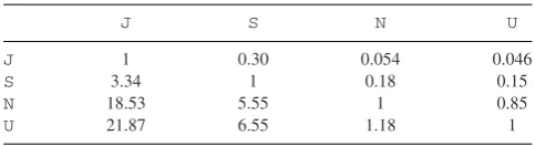
For our non-zero-mass substellar bodies, we adopted eight types of planets: Jupiter, Saturn, Uranus, Neptune (which we refer to as ‘giant planets’), and all of their analogues scaled down in mass by a ratio of MJupiter/M⊕ ≈317.8 (which we refer to as
‘terres-trial planets’). The mass scaling effectively transforms Jupiter into Earth, and the other giant planets into three sub-Earth mass compan-ions. The scaled-down planets allow us to provide direct dynamical comparisons while keeping the mass ratios amongst the planets the same. These terrestrial planets also arguably yielded the most
5Rarely has the future non-secular evolution of planetary systems
[image:4.595.45.286.320.363.2]Table 2. Mass ratios of different planets (J=Jupiter,S=Saturn,N= Nep-tune,U=Uranus). These ratios are equivalent to those of the planets which are scaled-down in mass ( ¯J, ¯S, ¯N, ¯U).
J S N U
J 1 0.30 0.054 0.046
S 3.34 1 0.18 0.15
N 18.53 5.55 1 0.85
U 21.87 6.55 1.18 1
interesting results. We adopted giant planet densities which reflect those of Jupiter, Saturn, Uranus and Neptune. The density of all the scaled-down planets was set to the density of the Earth.
We henceforth denote the giant planets asJ,S,U, N, and the terrestrial planets as ¯J, ¯S, ¯U, and ¯N. All of the planetary system com-binations that we adopted per simulation are presented in the ap-pendix. For perspective on the relative mass values, see Table2. Test particles are by definition massless, and can reasonably represent objects (whether they be planets, asteroids or pebbles) which are at least two or three orders of magnitude less massive than the non-zero mass bodies in the simulation. Also,MJupiter/M =9.54×10⁻⁴
and M⊕/M =3.00×10⁻⁶.
Our choices for initial orbital eccentricities, inclinations, orbital angles, and innermost semimajor axis follow those of previous stud-ies (Mustill et al.2014; Veras & G¨ansicke2015) and their justifica-tions are only briefly repeated here. All planets are assumed to be on initially circular orbits and have small inclinations randomly se-lected from a uniform distribution from−1◦to 1◦. Adopting strictly non-coplanar planets prevent an unnaturally high rate of planet– planet collisions, which occurred in Veras et al. (2013a). Imposing non-zero initial eccentricities would change (speed up) instability time-scales; we did not do so in order to facilitate comparisons with previous studies. The innermost planet semimajor axis was always set at 5 au to prevent AGB star–planet tides from playing a role in the evolution (see fig. 7 of Mustill & Villaver2012) before any po-tential instability occurs. Further, 5 au is a particularly appropriate value considering that Jupiter lies at 5.2 au from the Sun and is the closest of the four giant planets in our Solar system.
The much trickier initial parameter to determine was the initial spacing of the planets. For equal-mass planets, the link with initial spacing and instability time-scales has a now-substantial history (see Davies et al.2014for a review), particularly with the application of the mutual Hill radius as the separation unit. However, no widely used formalism exists with unequal-mass planets. Consequently, for lack of better proven alternatives, we applied the mutual Hill radius to our architectures here. Multiple definitions of this parameter exist: we adopted equation 4 of Smith & Lissauer (2009) in order to maintain consistency and provide meaningful comparisons with Veras & G¨ansicke (2015):
ai+1=ai
⎡ ⎣1+β
2
⎛
⎝ mi+mi+1
3
m+ik−=11mk
⎞ ⎠
1/3⎤
⎦
× ⎡ ⎣1− β
2
⎛
⎝ mi+mi+1
3
m+ik−=11mk
⎞ ⎠
1/3⎤
⎦
−1
. (1)
In this equation,aandmrefer to mass and initial semimajor axis, and the subscripts ascend in order of increasing distance from the star. The important quantityβis the number of mutual Hill radii. In order to determine meaningful values ofβfor the different architectures
we considered, we performed exploratory preliminary suites of sim-ulations. We found that a wide range (β=6–14) was necessary to implement depending on the architecture considered. The specific values used for each architecture are listed in TablesA1–A13.
Having established the planet locations, we then considered where potential test particles would reside. We distributed our 12 test particles uniformly in a ring at 2.5 au from the star. This choice is in the spirit, if not the details, of the asteroid belt. In our So-lar system, the So-largest objects in this belt (with sizes greater than 100 km) are unlikely to be influenced by solar GB radiation, and will neither be engulfed by the solar giant. Recall that these parti-cles could instead represent Mars, which also will survive the Sun’s post-main-sequence evolution, despite being located at about 1.5 au (Schr¨oder & Connon Smith2008).
2.4 Additional physics
Besides radiation, other physics that could play a role in planetary system evolution include star–planet tides and general relativity. A planet which is perturbed on an orbit with a pericentre that lies just outside of the Roche radius may be tidally circularized. The particulars of this process are highly dependent on the composition of the approaching planet and the evolutionary stage of the star; all our bodies are point-masses with no assumed composition. The variation in tidal circularization behaviour and time-scale due to composition is so great (Henning & Hurford2014) that any mean-ingful exploration would require a dedicated study, which we do not perform here. Our simulations here illustrate pre-conditions for this tidal interaction to occur.
General relativity changes the rate of the argument of periastron for close-in bodies, and hence can by itself trigger instability in multiplanet systems (e.g. Veras & Ford2010). Consequently, we have included the effects of general relativity in our simulations through our updated code.
2.5 Running time
We attempted to run all our simulations for 14 Gyr, which represents a Hubble time and is the current age of the Universe. We succeeded in over 90 per cent of cases, the exceptions (which are all noted in the appendix tables) being systems where a planet or test particle was perturbed close enough to the star to sufficiently slow down the simulations. We only report simulations which ran for at least 1.9 Gyr (recall that our star becomes a WD after about 1.5 Gyr), in order to give a flavour of what the evolution is like on all of the main-sequence, GB, and early WD phases.
3 R E S U LT S
We present results for over 450 simulations, and have visually in-spected the output and evolution of each one. They are partitioned into groups of up to four simulations such that each group member has the same (i) initial ordering and type of masses (such as ¯NU¯J¯S¯ in order of increasing distance from the star), and (ii) value ofβ. Within these groups the initial orbital angles and inclinations are different.
setting up future simulations if one has a desired outcome or set of initial conditions (perhaps based on a known exosystem) in mind.
In this section, we describe the data which is presented in the tables (Subsection 3.1), illustrate some representative and interest-ing examples (Subsection 3.2), list various system outcomes and behaviours which our simulations show to be possible tion 3.3), and analyse the general trends from the tables (Subsec-tion 3.4).
3.1 Description of table columns
In all tables, the first column (‘Sim #’) provides a designation for each simulation for easy reference. The second column (‘Setup’) provides the initial order and type of planets in each simulation. We reiterate thatJ,S,U, N, ¯J, ¯S, ¯U, and ¯N, respectively, refer to planets which have the same masses of Jupiter, Saturn, Uranus, Neptune, and versions of those planets with masses scaled down by a factor of about 318 (thereby transforming Jupiter into Earth). All simulations in TablesA1–A11contain four planets each. The last two tables (A12–A13) contain systems with four, six and eight planets. The third column (‘β’) refers to the number of mutual Hill radii between the planets, as defined from equation 4 of Smith & Lissauer (2009).
Starting from the fourth column (‘Unpack’), we characterize the timing of events in the evolution of the planetary system. We adopt designations for different phases of stellar evolution: MS (main se-quence), GB (giant branch), EWD (‘early white dwarf’ that corre-sponds to stars that have become WDs within the last 100 Myr), and LWD (‘late white dwarf’ stars which became WDs over 100 Myr ago). We split up the WD phase because the intense mass-loss at the tip of the AGB phase often triggers slightly delayed instabil-ity, which commonly manifests itself in WDs whose cooling age (the time since becoming a WD) is less than about 100 Myr. In ef-fect, such systems are dynamically resetting themselves and hence feature instability at ‘early’ times, just as we would expect from a planetary system recently born out of a Solar nebula. Precisely then, the MS phase corresponds to times between 0 and 1173.576 Myr, while the GB phase corresponds to times between 1173.576 and 1495.783 Myr. At 1495.783 Myr, the EWD phase begins and lasts until 1595.783 Myr. The star then spends the remainder of its life on the LWD phase.
The fourth column itself (‘Unpack’) displays the phase during which the system became unpacked. If the system never became unpacked, then the space is left blank. We define ‘unpacked’ as the moment that either (i) two non-zero mass planets cross orbits, or (ii) an instability occurs. We define instability as an occurrence when two bodies collide with one another, or one body escapes the system. The collision could come in the form of a star–planet collision (when the planet is said to be engulfed in the star) or a planet–planet collision. Note also that the moment of escape may occur several Myr after the actual interaction which triggered the movement, because the Hill ellipsoid of the system typically lies at about 105au from the star.
The fifth column (‘# Surv’) indicates the number of non-zero mass planets which remained in the system by the end of the simulation. Those planets which do not survive are characterized in the next three columns (‘Engulf’, ‘Eject’ and ‘Collision’), which indicate, respectively, when a planet intersects with the stellar radius, is ejected from the system, or hits another planet. Recall that the WD stellar radius is enhanced from its true value. The columns all indicate the phase in which an instability occurred, along with the planet(s) involved in the instability in the subscripts. The subscript
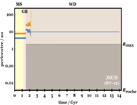
Figure 2. A characteristic outcome for the full-lifetime evolution of four giant planets: unpacking and instability on the main sequence, followed by stability. Note that the surviving two planets expand their orbits due to GB mass-loss at 1.49 Gyr. The values ofRmaxandRrocheon the right axis indicate the maximum stellar AGB radius (1.82 au) and an approximate value of the disruption radius of WDs (0.0059 au). Shown isJUUUsimulation #1-19 (TableA1).
numbers correspond to the planet order from the ‘Setup’ column. Each instability is indicated by a single listed entry. The subscripts in each ‘Collision’ entry indicate the two planets involved in the collision.
The column (‘<Rmax’) lists any non-zero mass planet that
sur-vived for the entire simulation and was perturbed into an orbit along the EWD or LWD phase whose pericentre was within the star’s max-imum AGB radius (1.82 au). The subscript indicates the smallest planet-WD distance that was achieved.
The column, labelled ‘TPs Eng’, does not exist in the final two tables (A12–A13). The column indicates when test particles were included in the simulations (a blank space means no test particles), and provides some information about them. The first and second numbers given are the amounts of test particles (out of 12) that were engulfed by the star during the EWD and LWD phases, respectively. The final column lists relevant notes which are in the table cap-tions.
3.2 Specific cases
Now, we present some specific examples of evolutionary sequences.
3.2.1 Standard giant planet evolution
Consider first simulation #1-19 (in TableA1), whose evolution is shown in Fig.2. The system initially consists of an inner Jupiter-mass planet (blue, at 5 au) followed by three Uranus-Jupiter-mass planets (JUUU), separated by β = 8. The system unpacks on the main sequence, and both the second and third planets (Uranuses) are ejected sometime during this phase. The two remaining planets have their orbits expanded due to mass-loss at the end of the GB phase, remaining stable through this process and for the remainder of the simulation. Neither achieved an orbit that took it to within 1.82 au (=Rmax) of the WD, and their pericentres remain nearly
Figure 3. Evolution of a Solar system analogue (JSUN) that immediately ejects Uranus and Neptune and keeps Saturn bound until the star is 2.2 Gyr old, which is 0.7 Gyr into the WD phase. Only Jupiter survives for this particular evolution, which is simulation #7-11 (TableA7).
3.2.2 Squeezed Solar system analogue – giant planets
Next consider a Solar system analogue architecture (JSUN and
β=7) from TableA7. Simulation #7–11, shown in Fig.3, features Neptune and Uranus being ejected at 10.3 and 18.5 Myr (effectively immediately), which is not discernable on the plot. The remaining Jupiter and Saturn mutually perturb each other so that their peri-centres vary significantly (over 1 au in each case) throughout the main sequence. The orbital expansion causes the two-planet sta-bility threshold (see Debes & Sigurdsson2002, Veras et al.2013a and Voyatzis et al.2013) to be passed or at least skirted, leading to delayed instability on the WD phase. The result is that at 2.2 Gyr, Saturn is ejected. Jupiter remains the lone survivor.
3.2.3 Solar system analogue – terrestrial planets
Alternatively, simulation #7-40 (β = 11, and Fig. 4) illustrates one evolutionary sequence for the scaled-down (by a mass factor of 318) versions of Jupiter, Saturn, Uranus and Neptune ( ¯JS¯U¯N¯) – effectively transforming them into terrestrial-mass planets. The system does not unpack until the EWD phase, but never becomes unstable. The resulting meandering causes the scaled-down Uranus (green) to achieve an orbital pericentre of just 2.47 au (less than half of any planet’s initial pericentre) at 6.67 Gyr.
3.2.4 Terrestrial planet pericentre repacking
Another example of a long-term stable terrestrial system, but one that becomes unpacked immediately, is from simulation #9–39 ( ¯UN¯J¯S¯ – blue, orange, green, red – from Table A9and left-hand panel of Fig.5). This simulation contains two notable features: (i) the inward radial incursion of¯Uto a few au at around 8 Gyr (the first such radial incursion during the entire evolution), and (ii) the ‘re-packing’ of the orbital pericentres beyond 8 Gyr. At this time, the system becomes orderly (but now in the order ¯UJ¯S¯N¯) and henceforth secularly evolves with well-defined and periodic oscillations.
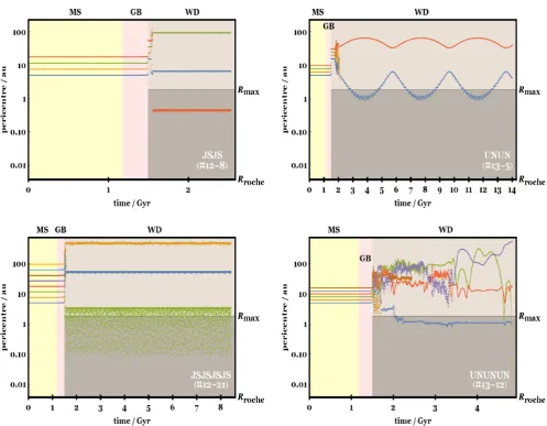
A second example of a repacked system, but one which becomes unstable, is illustrated in the right-hand panel of Fig.5( ¯UJ¯J¯J¯from simulation #2–24 of Table A2). Here, the unpacking occurs on
Figure 4. Unpacking of a set of terrestrial planets at the start of the WD phase. The planets ( ¯JS¯U¯N¯) are scaled-down versions of Jupiter, Saturn, Uranus and Neptune, with the mass reduced by a factor of about 318, which transforms Jupiter into the Earth. All four planets remain stable, meander, and survive until the end of the simulation. Shown is simulation #7–40 (TableA7).
the LWD phase, the smallest-mass planet is engulfed, and the two closest ¯Jplanets switch places.
3.2.5 Unpacked giant planets with test particles
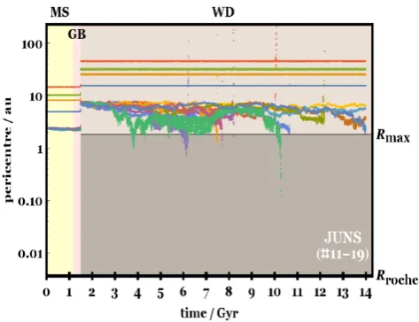
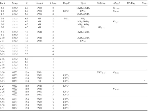
In reality, the above systems likely harbour Mars-like planets or asteroids in regions like our Solar system’s asteroid belt. Simulation #11-19 (JUNSandβ=9 from TableA11) contains 12 test particles located in initially circular orbits at 2.5 au. Fig.6shows the resulting evolution. The four giant planets remain packed and stable through the entire simulation, and have a non-disruptive effect on the test particles during the main-sequence and GB phases of evolution. However, on the WD phase, 8 of the 12 particles are lost. Seven are lost through ejections, all of which can be individually discerned on the plot (at times 6.22, 7.49, 7.71, 8.20, 10.08, 10.66 and 12.19 Gyr). One particle is engulfed inside of the WD (as indicated in the table) at 10.29 Gyr.
3.2.6 Deep radial incursions for almost equal-mass planets
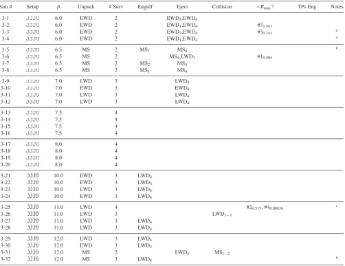
TablesA12andA13give details of simulations which contain al-most equal-mass planets, and therefore serve as a useful basis of comparison to both other simulations in this work and previous simulations of strictly equal-mass planets. The mass ratios of con-secutive planet pairs in the tables are just 3.34 and 1.18, respectively. In Fig.7, we display four simulations which show examples of how small ranges in planet mass within the same system can lead to deep radial incursions during the WD phase. Shown are four-, six-and eight-planet systems. In three of the cases (simulations #12-8, #12-21 and #13-12), the runs did not finish. Unpacking occurs on the WD phase in all cases, and instability results. The effects of tides (not modelled) might affect the green planets (which achieve pericentres of0.1 au) on the bottom plots.
3.3 The variety of system behaviours
[image:7.595.45.282.55.237.2]Figure 5. Two examples of unpacking then repacking, in both stable (left-hand panel) and unstable (right-hand panel) cases. Left-hand panel: immediate unpacking of a set of terrestrial planets, followed by a re-ordering and stable secular evolution from 8 Gyr onwards. The initial order of the planets is ¯UN¯J¯S¯but their orbits end up in the order ¯UJ¯S¯N¯. Shown is simulation #9–39 (TableA9). Right-hand panel: unpacking of ¯UJ¯J¯J¯on the WD phase, where the least massive, innermost, planet becomes engulfed and two of the other planets (orange and green) switch order. Shown is simulation #2-24 (TableA2).
Figure 6. A stable and unpacked set of giant planetsJUNSwith 12 test particles initially located at 2.5 au. Four particles survive, seven are ejected, and one enters the WD disruption radius at 10.29 Gyr. All these events are visible on the plot. Shown is simulation #11-19 (TableA11).
first consider the rich variety of behaviours and outcomes seen in the simulations and simply list what is possible from full-lifetime evolution for clarity.
(i) Unpacking (defined as crossing orbits or planet loss) may occur during any phase of stellar evolution, or not at all.
(ii) Unpacking through crossing orbits does not necessarily lead to instability (defined as planet loss from collisions or ejections).
(iii) Unpacking during one phase can lead to instability at a later phase.
(iv) Planet engulfment into the star, planet–planet collisions and ejections may all occur during any phase.
(v) Two systems with identical initial numbers, masses and sep-arations of planets can be unpacked at different phases and lose different numbers of planets.
(vi) Any total number of planets may be lost.
(vii) Planets which are formed when the star arrives on the main sequence at distances well outside of the maximum AGB stellar radius can be perturbed on the WD phase to distances well within the maximum AGB stellar radius.
(viii) Test particles which initially reside within the orbits of four giant planets can survive for the entire simulation duration even when the giant planets unpack and/or become unstable.
3.4 General trends
In this section, we present the crux of our results and some trends with applications beyond this work.
3.4.1 Relating toβ
(i) Unpacking tends to occur at later stellar phases as β is increased. This correlation is typically strong but by no means monotonic. For example, consider simulations #8-1 through #8-32 (TableA8), whereβ is increased from 6.0 to 9.5. For a weaker correlation, instead see simulations #9-1 through #9-32 (TableA9), and for a better correlation, see simulations #4-1 through #4-24 (TableA4). See Fig.8for a visual representation of the correlation (although the tables themselves might be clearer).
(ii) Mapping a particular value ofβto the phase at which one could expect unpacking is architecture-dependent. Compare for ex-ample, the simulations withβ=7.0 across all of the tables.
(iii) Terrestrial-mass planets (effectively, ¯J, ¯S, ¯U, and ¯N) at a given
βwill unpack at an earlier phase than their giant-planet counterparts (implied from Tables A1–A11and Fig. 8) due to the additional dependence of stability time-scale on mass, which is not captured by the Hill radius (e.g. Chambers, Wetherill & Boss1996; Faber & Quillen2007; Mustill et al.2014).
3.4.2 Relating to engulfments, ejections and collisions
[image:8.595.47.284.304.486.2]mass terrestrial planet is engulfed into the WD in the majority of cases (see e.g. Fig.5).
(ii) In-between these two regimes (giant planets and terrestrial planets) are the low-mass giant planets, or ice giants, withUNUN,
UNUNUNandUNUNUNUN(TableA13). Only for these systems do unstable events appear to be roughly evenly distributed amongst ejections, engulfments and planet–planet collisions. For simulations #13-12 to #13-17, the lack of planet–planet collisions might be due to the truncated duration of those simulations and/or neglecting WD-planet tides.
(iii) Physically, the trends in the above two bullet points are un-derstandable in terms of the Safronov number (Safronov & Zvjagina 1969), which is the square of the ratio of the surface escape speeds to the planetary orbital speeds. As this ratio increases, the frequency of ejections increases. This ratio is approximately unity for Earth-like planets at 20 au, but about 40 for Jupiters at the same separation.
(iv) The commonality of planet–planet collisions in terrestrial-planet systems implies that those systems should contain more de-bris and newly generated asteroids than giant planet systems.
(v) The unpacking of systems with four giant planets prefer-entially (80 per cent) results in the survival of two planets. This percentage would be 90 per cent if not for theUNJSand NUJS
architectures (TablesA9andA10), which do not follow this trend. In these architectures, either the Uranus or Neptune is typically ejected but the other survives.
(vi) The unpacking of systems with four terrestrial planets in-stead preferentially (55 per cent) results in the survival of three planets, and in 30 per cent of cases retains all four planets. This stark difference from the giant-planet case is likely related to the in-ability for close encounters in terrestrial-planet systems to be strong enough to cause ejections.
(vii) Unpacked terrestrial-planet architectures which retain all planets are typically aperiodic in their resulting orbital variations (see e.g. Fig.4). This feature is particularly noteworthy because these systems produce an ever-changing dynamic environment, which may tap into different reservoirs of WD pollutants at dif-ferent cooling ages.
(viii) When architectures contain one most massive planet (as opposed to two or more), as in TablesA1,A4,A7–A11, that planet isneverejected nor engulfed into the star. Physically, the reason is due to conservation of angular momentum and energy, even though the system energy is strictly not conserved during GB mass-loss.
(ix) For systems that contain exactly two most massive planets, those planets rarely are ejected or engulfed into the star. This ten-dency holds true for every single system simulated with Jupiters, Uranuses and their scaled equivalentsJUUJ, ¯JU¯U¯J¯,UJJU, ¯UJ¯J¯U¯ (TablesA5andA6). ForJSJS(TableA12), where the difference in planet mass is much less (ratio of 3 as opposed to 22), there is only one exception (simulation #12-6). ForUNUN(TableA13), there are two exceptions.
(x) Rarely (6.6 per cent) does unpacking of four-planet systems allow for at least one of the planets to eventually achieve an orbital pericentre within the maximum AGB radius of 1.8 au, in contrast to the equal planet-mass case (Veras & G¨ansicke2015).
(xi) Deep radial incursions are most common for the unequal-mass systems which are closest to the equal-unequal-mass case, namely the UJJJ, ¯UJ¯J¯J¯, JJJU, ¯JJ¯J¯U¯, JSJS and UNUN cases (Tables A2, A3, A12and A13). The reason for the similarity is in the first four cases when one ignores/ejects the Uranus, and in the latter two cases because the range of their masses is small. In that respect, the greatest incidence of inward radial incursions oc-curs for theUNUNarchitecture, because with a mass ratio of 1.18
between adjacent pairs of planets, the system effectively contains equal-mass planets.
(xii) Increasing the number of planets in a system increases the incidence for deep inward radial incursions, as well as consistently changing dynamical architectures, similar to the equal-planet mass case.
3.4.3 Relating to test particles
(i) Unpacking of the non-zero mass planets enhances prospects for WD engulfment of test particles, which can reasonably represent Mars-like planets or large asteroids.
(ii) Even with the tiny sample sizes adopted here (12 test parti-cles per simulation, as constrained by computational limitations), enough are engulfed by WDs (263 out of a total 1024) to suggest both that this process is crucial and that higher resolution studies are needed to detect discernable trends.
4 D I S C U S S I O N
In order to place our results in context, we will discuss the conse-quences for polluted WD systems and consider the links to three outstanding observational constraints: (i) pollution rate with WD cooling age, (ii) accumulated metal pollution in non-DA WD, and (iii) the WDs 1145+017 system. We will also discuss the implica-tions of so many ejecimplica-tions for the purported free-floating population of planets within the Milky Way, and how our simulations may be linked to chaos.
4.1 Consequences for polluted WD systems
Our simulations clearly demonstrate that planet engulfment into WD is a rare phenomenon (8.8 per cent across all simulations), in line with the findings of the equal-planet mass studies of Veras et al. (2013a), Mustill et al. (2014) and Veras & G¨ansicke (2015). A much more likely pollution reservoir is the test particles, which we have shown can easily be engulfed in the WD, in line with the one-planet studies of Bonsor, Mustill & Wyatt (2011), Debes et al. (2012) and Frewen & Hansen (2014). The difference here is that multiple planets provide the opportunity for a constantly changing dynamic environment, which is not the case in one-planet systems.6 Consequently, multiple-planet systems are much more
likely to explain high rates of pollution at different cooling ages by accessing and perturbing different reservoirs of material (asteroids, fragments, dust) at different times and/or different locations.
Here, we have characterized this environment by sampling sys-tems of unequal-mass planets, where the planet masses differ by a factor of up to about 20. We found that this inequality has clear but second-order effects on the dynamics; the first-order effects are determined by what types of planets are involved in the unpack-ing: terrestrial or giant. For giant planets, crossing orbits trigger violent encounters between giant planets, but still typically cause the system to settle into a periodic secular state (see Fig.2and the upper-left panel of Fig.7).For terrestrial planets, fully 30 per cent of our simulations become unpacked (orbit-crossed) but never un-stable (featuring engulfments, ejections or collisions). The result is
6Stellar flybys can change the environment regardless of the number of
planets, but typically 10 Gyr needs to pass before a flyby achieves a close encounter within a few hundred astronomical units (Zakamska & Tremaine
Figure 7. Deep radial incursions due to unpacking on the WD phase of similar-mass giant planets in the systemsJSJS(upper-left panel, simulation #12-8), JSJSJSJS(lower-left panel, simulation #12-21),UNUN(upper-right panel, simulation #13-5) andUNUNUN(lower-right panel, simulation #13-12). Tides are unlikely to play a role in the upper panels, but might affect the evolution of the green planets in the lower panels. The striking behaviour seen here is characteristic of the simulations from TablesA12andA13.
a highly dynamic environment, where the planetary orbitsmeander
(see Fig.4), which is much more conducive to effective scattering at late ages.
4.2 Correlation with cooling age
Our choice of dividing up the WD phase into separate EWD and LWD phases was partly motivated by our simulation results, be-cause a WD cooling age of 100 Myr is a representative end value for the epoch of rapid post-main-sequence planetary instability (see e.g. Fig.9). However, this value is also sensible from an observa-tional point of view. The cooling ages of the WDs in Koester et al. (2014) are all below 200 Myr, while WD atmospheric properties can significantly change at cooling ages of∼500 Myr (see their fig. 8, middle panel). Therefore, a cut at cooling ages of a few 100 Myr is a natural way to separate samples observationally.
However, observations which have been obtained so far indicate that the accretion rate of metals on to WD atmospheres remains a flat function of WD cooling age (fig. 4 of Koester et al.2014). Ex-plaining pollution at late times (after many Gyr of WD evolution) is challenging because instability on the WD phase is partially
trig-gered by the increase in system stochasticity due to RGB and AGB mass-loss (Voyatzis et al.2013), preferentially leading to instabil-ities at early cooling ages. Fig.9emphasizes this tendency, even though this study does not attempt to model a realistic population synthesis (which is anyway beyond current computational means). Recent and ongoing work is exploring potential ways of polluting WDs at late cooling ages. One possibility is through the change in orbits of wide binary stellar companions due to Galactic tides after, and only after, one of the components has become a WD (Bonsor & Veras2015). However, the majority of known polluted WDs do not appear to harbour wide-orbit companions. Another possibility is through Lidov–Kozai secular evolution amongst multiple planets, such that the close encounters between planets and WDs first occur only after cooling ages of several Gyr (Petrovich & Mu˜noz, in preparation). Finally, an extant fragment field from planet–planet collisions may persist for several Gyr before being thrust towards the WD (Shannon et al., in preparation).
Figure 8. The phases at which unpacking occurs with respect toβfor the eight architectures given in the legend. Each point represents one simulation. Generally, asβis increased, unpacking occurs during later phases, although the relationship is not monotonic. The terrestrial-sized planets (open squares) generally require higher values ofβthan giant planets (dots) to achieve the same results. Unpacking during the GB phase is rare.
and instances when a planet or test particle approaches the vicinity of the WD. Meandering of low-mass (terrestrial-like) planets provides a dynamic environment with which extant debris or fragments may be perturbed to the WD at all ages. Our results show that mass equality amongst planets is not a requirement for late-age pollution, and is not in fact even preferential for producing instabilities at late ages.
4.3 Accumulated metals in convection zone
WDs with deep convection zones (usually containing helium-dominated atmospheres) retain a measurable record of the accreted planetary debris over a span of time up to a few Myr (see fig. 1 of Wyatt et al.2014). Fig.6of Veras (2016) illustrates the amount of mass accreted for three different samples from Farihi et al. (2010), Girven et al. (2012) and Xu & Jura (2012).
The accumulated mass ranges from the mass of Phobos to that of Pluto, and may have been accrued by a single object or a collection of bodies. Distinguishing these two possibilities is not possible observationally. From theory, we may determine the likelihood of a sequence of bodies impacting the WD or entering its Roche radius within 1 Myr. However, the sample size of the test particles in our simulations here (12 per simulation) was too small to determine impact frequency for a given architecture.
The accretion itself might represent a combination of a ‘con-tinuous’ stream of small particles from a surrounding disc and a ‘stochastic’ agglomeration of larger particles from elsewhere in the system. Wyatt et al. (2014) showed that the size boundary between these two regimes is approximately 35 km, and further constrained the potential size distribution of this accreted material, ruling out a mono-mass distribution. Further, discs have been detected around only a few per cent of polluted WDs (Farihi, Jura & Zuckerman 2009; Girven et al.2011; Steele et al.2011), although the actual fraction is likely greater than half (Bergfors et al.2014). Conse-quently, stochastic accretion is likely to play a role in many of these systems. The mechanics of impact into WD atmospheres indicates that the parameter space may be split into sublimation, fragmenta-tion and ablafragmenta-tion regimes (Brown et al., in preparafragmenta-tion) such that the details of the deposition are complex, but the end result is still metals in the convection zone.
4.4 WD 1145+017
The WD 1145+017 planetary system represents the only example of a metal-polluted WD with a surrounding debris disc composed of both dust and gas and disintegrating objects (asteroids, planets, or something in-between) detected by transit photometry. In this respect, the system provides a self-consistent snapshot of the disc
[image:11.595.48.541.506.695.2]formation and accretion process that is likely to take place at other metal-polluted WDs, and confirms long-standing theories (Graham et al.1990; Jura2003; Bear & Soker2013).
The system was announced by Vanderburg et al. (2015), who presented transit curves that illustrated that up to six objects with orbital periods of about 4.5–4.9 h are in the process of disintegrating and producing dust. They found that the dominant orbital period is closer to 4.5 h, which places the objects near the WD’s Roche radius, assuming that the objects are rubble-piles like the asteroids seen in the Solar system. The sizes of these objects are poorly constrained, and could range anywhere from∼1 to 1000 km. We will henceforth refer to them as planetesimals.
Follow-up observations came quickly (Croll et al.2016; G¨ansicke et al.2016; Rappaport et al.2016; Xu et al.2016). Xu et al. (2016) detected gas in the debris disc and showed that the WD atmosphere is polluted with 11 heavy elements. Croll et al. (2016) performed multiwavelength observations that illustrated the number of plan-etesimals disintegrating is likely more than one, and helped confirm that the planetesimals harbour an orbital period of about 4.5 h rather than a value closer to 4.9 h. Further follow-up was provided by G¨ansicke et al. (2016), who used high-speed photometry and observations of the system from 2015 Nov–Dec to reveal that at least six planetesimals are breaking up, and that they share the same near-circular orbit with orbital periods of about 4.4930 h. Rappa-port et al. (2016) most recently detected drifting features which they postulate are fragments that broke off from a single progenitor.
Our results, along with those of Bonsor et al. (2011), Debes et al. (2012), Frewen & Hansen (2014) and Veras & G¨ansicke (2015), demonstrate that the progenitor of the planetesimals in WD 1145+017 may be a large asteroid that was scattered in the vicinity of the WD. The scattering may be caused by one planet (Bonsor et al. 2011; Debes et al.2012; Frewen & Hansen2014) or multiple planets (this paper). Alternatively, the progenitor may be a moon (Payne et al.2016), or a small (terrestrial) planet, as shown by both Veras & G¨ansicke (2015) and this paper. Multiple planets can scatter a test particle into a transit-detectable orbit, even if the planets themselves never unpack (Fig.6). We note that a Solar system analogue, with
JSUNand asteroids or a Mars, can easily generate the progenitor of the planetesimals in WD 1145+017. The mass of the progenitor remains unconstrained (Veras, Marsh & G¨ansicke2016).
Our simulations suggest that WD 1145+017 is not unique in hosting transiting planetesimals. Many possible multiplanet scenar-ios can perturb test particles into the Roche radius of the WD; we have just scratched the surface.
4.5 Free-floating planet population contribution
A brief inspection of the tables in the appendix reveal a pre-ponderance of planetary ejections. This feature, just like for the equal-mass planet case (Veras et al.2013a; Mustill et al.2014), and even the single-planet case (Veras et al.2011; Veras & Tout2012; Veras et al.2014a), help establish that planetary ejection is an ubiq-uitous feature of post-main-sequence systems. Consequently, these ejections make a contribution to the free-floating planet population. How this contribution compares to that due to the dynamical activity which accompanies planetary formation and protoplane-tary disc dissipation (e.g. Rasio & Ford1996; Levison, Lissauer & Duncan1998; Marzari & Weidenschilling2002; Veras & Ar-mitage2005,2006; Raymond et al.2011,2012; Matsumura, Ida & Nagasawa2013) is not yet clear, primarily because our observational knowledge of exoplanets beyond 5 au is sparse. Nevertheless, we have an extraordinary observational estimate on the total number of
free-floating giant planets in the Milky Way: nearly two for every main-sequence star (Sumi et al.2011). If future observations affirm this result, then identifying the origin of so many free-floaters will remain a major question in planetary science. Planetary scattering alone with single stars on the main sequence cannot explain this population (Veras & Raymond 2012), and the contribution from scattering in binary systems has not yet been quantified, despite studies such as Sutherland & Fabrycky (2016) and Smullen, Kratter & Shannon (2016).
We caution that although ejections were perhaps common amongst the currently observed population of WDs (as illustrated by this study), the resulting contribution to the currently observed free-floating planet population as reported by Sumi et al. (2011) would be of the order of 1 per cent (Veras & Raymond2012). Each WD progenitor system would need to have harboured tens of gi-antplanets to achieve the Sumi et al. (2011) result. This number is thought to be too large, despite the likely positive correlation between stellar mass and planet multiplicity (Kennedy & Kenyon 2008; Andrews et al.2013), partly because of the extreme case HR 8799, which contains (just) four giant and packed planets (Marois et al.2010). HR 8799 also provides a representative glimpse into the past of WD planetary systems because of its A-star host.
4.6 Linking meandering with chaotic behaviour
The phenomenon we refer to as meandering is linked to the stochas-ticity of the system. The vast literature on chaos indicators in grav-itational point-mass exoplanetary systems utilizes a wide variety of techniques in order to characterize, in part, how close the system is to instability at different times. Linking these indicators toN-body integrations – particularly long-term integrations – remains chal-lenging (e.g. Veras, Antoniadou & G¨ansicke, in preparation) but may provide key constraints.
Only two published dedicated post-main-sequence studies of which we are aware have attempted to link evolution with stochas-ticity at the beginning and end of mass-loss (Adams, Anderson & Bloch2013; Voyatzis et al.2013). Both studies use the classi-cal Lyapunov exponent as their chaos indicators, and consider two planets. Their work brings attention to subtleties which indicate that dedicated studies on chaos would be beneficial. We frame these subtleties as the following questions. (i) What metric (e.g. Carte-sian coordinate, eccentricity), and corresponding reference frame or coordinate system, would provide the most representative link to instability? (ii) How does one combine chaos indicators for multi-planet systems, particularly after close encounters, and after one or more of the planets is lost from the system? (iii) What chaos indi-cators are affected by the Hamiltonian-breaking physics of stellar mass-loss, and how do different mass-loss prescriptions affect the usefulness of a particular indicator?
Although these questions are too big to tackle here, our simu-lations provide a template on which future dedicated studies may make useful comparisons.
5 C O N C L U S I O N S
(i) unlike in the giant planet case, terrestrial-planet unpacking (orbit crossing) often does not trigger instability (engulfments, ejec-tions and collisions), and provides a more dynamic, constantly shift-ing evolution throughout the WD phase; this result is independent of the mass variation amongst planets.
(ii) The smaller the dispersion in planetary mass, the closer those planets may be perturbed towards the WD.
(iii) Giant planet systems preferentially feature ejections whereas terrestrial-planet systems preferentially feature planet–planet colli-sions. Consequently, we expect more potentially polluting debris to exist in terrestrial-planet systems.
(iv) Prospects for unpacking roughly increase asβ increases, although this relationship is not monotonic and dependent on the considered architecture.
Ultimately, how planets behave at different phases of evolution will crucially determine the subsequent evolution of the smaller bodies in those systems, bodies which are most likely the progen-itors of WD pollution and planetesimals such as those observed disintegrating around WD 1145+017.
AC K N OW L E D G E M E N T S
We thank Fred C. Adams for an astute referee report. DV and BTG have received funding from the European Research Council under the European Union’s Seventh Framework Programme (FP/2007-2013)/ERC Grant Agreement no. 320964 (WDTracer). AJM ac-knowledges support from grant number KAW 2012.0150 from the Knut and Alice Wallenberg foundation and the Swedish Research Council (grant 2011-3991).
R E F E R E N C E S
Adams F. C., Anderson K. R., Bloch A. M., 2013, MNRAS, 432, 438 Andrews S. M., Rosenfeld K. A., Kraus A. L., Wilner D. J., 2013, ApJ, 771,
129
Barclay T., Quintana E. V., Adams F. C., Ciardi D. R., Huber D., Foreman-Mackey D., Montet B. T., Caldwell D., 2015, ApJ, 809, 7
Bear E., Soker N., 2013, New Astron., 19, 56
Bergfors C., Farihi J., Dufour P., Rocchetto M., 2014, MNRAS, 444, 2147 Bonsor A., Veras D., 2015, MNRAS, 454, 53
Bonsor A., Mustill A. J., Wyatt M. C., 2011, MNRAS, 414, 930 Campante T. L. et al., 2015, ApJ, 799, 170
Casewell S. L., Dobbie P. D., Napiwotzki R., Burleigh M. R., Barstow M. A., Jameson R. F., 2009, MNRAS, 395, 1795
Cassan A. et al., 2012, Nature, 481, 167
Catal´an S., Isern J., Garc´ıa-Berro E., Ribas I., 2008, MNRAS, 387, 1693 Chambers J. E., 1999, MNRAS, 304, 793
Chambers J. E., Wetherill G. W., Boss A. P., 1996, Icarus, 119, 261 Croll B. et al., 2016, preprint (arXiv:1510.06434)
Davies M. B., Adams F. C., Armitage P., Chambers J., Ford E., Morbidelli A., Raymond S. N., Veras D., 2014, in Beuther H., Klessen R. S., Dullemond C. P., Henning T., eds, Protostars and Planets VI. Univ. Arizona Press, Tucson, AZ, p. 787
Debes J. H., Sigurdsson S., 2002, ApJ, 572, 556 Debes J. H., Walsh K. J., Stark C., 2012, ApJ, 747, 148
Dong R., Wang Y., Lin D. N. C., Liu X.-W., 2010, ApJ, 715, 1036 Dufour P. et al., 2007, ApJ, 663, 1291
Duncan M. J., Lissauer J. J., 1998, Icarus, 134, 303 Faber P., Quillen A. C., 2007, MNRAS, 382, 1823
Falcon R. E., Winget D. E., Montgomery M. H., Williams K. A., 2010, ApJ, 712, 585
Farihi J., 2016, New Astron. Rev., in press
Farihi J., Jura M., Zuckerman B., 2009, ApJ, 694, 805
Farihi J., Barstow M. A., Redfield S., Dufour P., Hambly N. C., 2010, MNRAS, 404, 2123
Frewen S. F. N., Hansen B. M. S., 2014, MNRAS, 439, 2442 G¨ansicke B. T. et al., 2016, ApJ, 818, L7
Gentile Fusillo N. P., G¨ansicke B. T., Greiss S., 2015, MNRAS, 448, 2260 Girven J., G¨ansicke B. T., Steeghs D., Koester D., 2011, MNRAS, 417, 1210 Girven J., Brinkworth C. S., Farihi J., G¨ansicke B. T., Hoard D. W., Marsh
T. R., Koester D., 2012, ApJ, 749, 154
Gomes R., Levison H. F., Tsiganis K., Morbidelli A., 2005, Nature, 435, 466
Graham J. R., Matthews K., Neugebauer G., Soifer B. T., 1990, ApJ, 357, 216
Guillochon J., Ramirez-Ruiz E., Lin D., 2011, ApJ, 732, 74 Henning W. G., Hurford T., 2014, ApJ, 789, 30
Hurley J. R., Pols O. R., Tout C. A., 2000, MNRAS, 315, 543
Izidoro A., Raymond S. N., Morbidelli A., Winter O. C., 2015, MNRAS, 453, 3619
Jura M., 2003, ApJ, 584, L91
Kalirai J. S., Hansen B. M. S., Kelson D. D., Reitzel D. B., Rich R. M., Richer H. B., 2008, ApJ, 676, 594
Kennedy G. M., Kenyon S. J., 2008, ApJ, 673, 502 Kepler S. O. et al., 2015, MNRAS, 446, 4078 Kepler S. O. et al., 2016, MNRAS, 455, 3413 Kleinman S. J. et al., 2013, ApJS, 204, 5
Koester D., G¨ansicke B. T., Farihi J., 2014, A&A, 566, A34 Levison H. F., Lissauer J. J., Duncan M. J., 1998, AJ, 116, 1998
Levison H. F., Morbidelli A., Tsiganis K., Nesvorn´y D., Gomes R., 2011, AJ, 142, 152
Liebert J., Bergeron P., Holberg J. B., 2005, ApJS, 156, 47
Liu S.-F., Guillochon J., Lin D. N. C., Ramirez-Ruiz E., 2013, ApJ, 762, 37 Luhman K. L., Burgasser A. J., Bochanski J. J., 2011, ApJ, 730, L9 Marois C., Zuckerman B., Konopacky Q. M., Macintosh B., Barman T.,
2010, Nature, 468, 1080
Marzari F., Weidenschilling S. J., 2002, Icarus, 156, 570 Matsumura S., Ida S., Nagasawa M., 2013, ApJ, 767, 129
Morbidelli A., Levison H. F., Tsiganis K., Gomes R., 2005, Nature, 435, 462
Mustill A. J., Villaver E., 2012, ApJ, 761, 121
Mustill A. J., Marshall J. P., Villaver E., Veras D., Davis P. J., Horner J., Wittenmyer R. A., 2013, MNRAS, 436, 2515
Mustill A. J., Veras D., Villaver E., 2014, MNRAS, 437, 1404 Nordhaus J., Spiegel D. S., 2013, MNRAS, 432, 500
O’Brien D. P., Walsh K. J., Morbidelli A., Raymond S. N., Mandell A. M., 2014, Icarus, 239, 74
Paxton B., Bildsten L., Dotter A., Herwig F., Lesaffre P., Timmes F., 2011, ApJS, 192, 3
Paxton B. et al., 2015, ApJS, 220, 15
Payne M. J., Veras D., Holman M. J., G¨ansicke B. T., 2016, MNRAS, 457, 217
Pierens A., Raymond S. N., 2011, A&A, 533, A131 Portegies Zwart S., 2013, MNRAS, 429, L45 Pu B., Wu Y., 2015, ApJ, 807, 44
Rappaport S., Gary B. L., Kaye T., Vanderburg A., Croll B., Benni P., Foote J., 2016, preprint (arXiv:1602.00740)
Rasio F. A., Ford E. B., 1996, Science, 274, 954 Raymond S. N. et al., 2011, A&A, 530, A62 Raymond S. N. et al., 2012, A&A, 541, A11
Reffert S., Bergmann C., Quirrenbach A., Trifonov T., K¨unstler A., 2015, A&A, 574, A116
Safronov V. S., Zvjagina E. V., 1969, Icarus, 10, 109 Schr¨oder K.-P., Connon Smith R., 2008, MNRAS, 386, 155 Schr¨oder K.-P., Cuntz M., 2005, ApJ, 630, L73
Sigurdsson S., Richer H. B., Hansen B. M., Stairs I. H., Thorsett S. E., 2003, Science, 301, 193
Smith A. W., Lissauer J. J., 2009, Icarus, 201, 381
Smullen R. A., Kratter K. M., Shannon A., 2016, ApJ, submitted Steele P. R., Burleigh M. R., Dobbie P. D., Jameson R. F., Barstow M. A.,
Sumi T. et al., 2011, Nature, 473, 349
Sutherland A. P., Fabrycky D. C., 2016, ApJ, 818, 6
Tremblay P.-E., Ludwig H.-G., Steffen M., Freytag B., 2013, A&A, 559, A104
Tsiganis K., Gomes R., Morbidelli A., Levison H. F., 2005, Nature, 435, 459
Vanderburg A. et al., 2015, Nature, 526, 546 Veras D., 2016, R. Soc. Open Sci., 3, 150571 Veras D., Armitage P. J., 2005, ApJ, 620, L111 Veras D., Armitage P. J., 2006, ApJ, 645, 1509 Veras D., Evans N. W., 2013, MNRAS, 430, 403 Veras D., Ford E. B., 2010, ApJ, 715, 803 Veras D., G¨ansicke B. T., 2015, MNRAS, 447, 1049 Veras D., Moeckel N., 2012, MNRAS, 425, 680 Veras D., Raymond S. N., 2012, MNRAS, 421, L117 Veras D., Tout C. A., 2012, MNRAS, 422, 1648
Veras D., Wyatt M. C., Mustill A. J., Bonsor A., Eldridge J. J., 2011, MNRAS, 417, 2104
Veras D., Mustill A. J., Bonsor A., Wyatt M. C., 2013a, MNRAS, 431, 1686 Veras D., Hadjidemetriou J. D., Tout C. A., 2013b, MNRAS, 435, 2416 Veras D., Evans N. W., Wyatt M. C., Tout C. A., 2014a, MNRAS, 437, 1127 Veras D., Leinhardt Z. M., Bonsor A., G¨ansicke B. T., 2014b, MNRAS, 445,
2244
Veras D., Jacobson S. A., G¨ansicke B. T., 2014c, MNRAS, 445, 2794
Veras D., Shannon A., G¨ansicke B. T., 2014d, MNRAS, 445, 4175 Veras D., Eggl S., G¨ansicke B. T., 2015a, MNRAS, 451, 2814 Veras D., Eggl S., G¨ansicke B. T., 2015b, MNRAS, 452, 1945 Veras D., Marsh T. R., G¨ansicke B. T., 2016, MNRAS, submitted Villaver E., Livio M., Mustill A. J., Siess L., 2014, ApJ, 794, 3
Voyatzis G., Hadjidemetriou J. D., Veras D., Varvoglis H., 2013, MNRAS, 430, 3383
Walsh K. J., Morbidelli A., Raymond S. N., O’Brien D. P., Mandell A. M., 2011, Nature, 475, 206
Winn J. N., Fabrycky D. C., 2015, ARA&A, 53, 409
Wyatt M. C., Farihi J., Pringle J. E., Bonsor A., 2014, MNRAS, 439, 3371 Xu S., Jura M., 2012, ApJ, 745, 88
Xu S., Jura M., Dufour P., Zuckerman B., 2016, ApJ, 816, L22 Zakamska N. L., Tremaine S., 2004, AJ, 128, 869
Zuckerman B., Koester D., Reid I. N., H¨unsch M., 2003, ApJ, 596, 477 Zuckerman B., Melis C., Klein B., Koester D., Jura M., 2010, ApJ, 722, 725
A P P E N D I X A : S I M U L AT I O N DATA TA B L E S
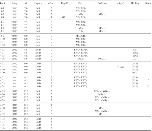
Table A1. Summary of results forJUUUand ¯JU¯U¯U¯. We summarize the column definitions (see Section 3.1 for a full description) as:Sim #: simulation designation.Setup: planet type and order from closest to furthest. Overbars denote a mass reduction by a factor of 318.β: number of mutual Hill radii.Unpack: stellar phase during which unpacking occurs.# Surv: number of surviving planetsEngulf: planets (identified in subscripts in number order from closest to furthest) which intersect the star’s surface or Roche radius, and the phase when the engulfment occurs.Eject: planets (identified in subscripts in number order from closest to furthest) which are ejected from the system, and the phase when the ejection occurs.Collision: planets (identified in subscripts in number order from closest to furthest) which collide with one another, and the phase when the collision occurs.<Rmax: surviving planets (identified in number order from closest to furthest) which achieve an orbital pericentre less than 1.82 au during the EWD or LWD phase; the minimum pericentre is provided in the subscript.
TPs Eng: number of test particles out of 12 which are engulfed in the EWD/LWD phases.Phase abbreviations: MS=main sequence, GB=giant branch, EWD=WD with 0–100 Myr cooling, LWD=WD beyond 100 Myr cooling.
Sim # Setup β Unpack # Surv Engulf Eject Collision <Rmax? TPs Eng Notes
1-1 JUUU 6.0 MS 2 MS2,MS3
1-2 JUUU 6.0 MS 2 MS3 MS1−2
1-3 JUUU 6.0 MS 2 MS2,MS3
1-4 JUUU 6.0 MS 2 MS2,MS3
1-5 JUUU 6.5 MS 2 MS3,MS4
1-6 JUUU 6.5 MS 2 MS3,MS4
1-7 JUUU 6.5 MS 2 MS3 MS1−4
1-8 JUUU 6.5 MS 2 MS2,MS3
1-9 JUUU 7.0 MS 2 MS2,MS3
1-10 JUUU 7.0 MS 2 MS2,MS3
1-11 JUUU 7.0 MS 2 MS3,MS4
1-12 JUUU 7.0 MS 2 MS2 MS3−4
1-13 JUUU 7.5 MS 2 MS2,MS4
1-14 JUUU 7.5 EWD 2 EWD3,EWD4
1-15 JUUU 7.5 EWD 2 EWD3,EWD4
1-16 JUUU 7.5 EWD 2 EWD2,EWD4
1-17 JUUU 8.0 MS 2 MS3,EWD4 d
1-18 JUUU 8.0 MS 2 MS3,MS4
1-19 JUUU 8.0 MS 2 MS2,MS3
1-20 JUUU 8.0 MS 2 MS3,MS4
1-21 JUUU 8.5 EWD 2 EWD3,EWD4 (0/0)
1-22 JUUU 8.5 LWD 2 LWD2,LWD4 (0/0)
1-23 JUUU 8.5 LWD 2 LWD2,LWD3 (0/4)
1-24 JUUU 8.5 LWD 2 LWD2,LWD4 (0/0)
1-25 JUUU 9.0 LWD 2 LWD2,LWD3 (0/0)
1-26 JUUU 9.0 EWD 2 EWD3,EWD4 (0/0)
1-27 JUUU 9.0 EWD 2 EWD3,EWD4 (3/2)
1-28 JUUU 9.0 EWD 2 EWD3,EWD4 (2/0)
1-29 JUUU 9.5 4 (0/0)
1-30 JUUU 9.5 4 (0/0)
1-31 JUUU 9.5 4 (0/0)
1-32 JUUU 9.5 4 (0/0)
1-33 J¯U¯U¯U¯ 10.0 MS 3 MS1−4
1-34 J¯U¯U¯U¯ 10.0 MS 2 MS2−3,MS1−2
1-35 J¯U¯U¯U¯ 10.0 MS 3 MS1−2
1-36 J¯U¯U¯U¯ 10.0 MS 2 MS1−4,MS1−2
1-37 J¯U¯U¯U¯ 11.0 MS 3 MS3−4
1-38 J¯U¯U¯U¯ 11.0 MS 2 MS1−2,MS3−4
1-39 J¯U¯U¯U¯ 11.0 MS 2 MS1−3,LWD1−2
1-40 J¯U¯U¯U¯ 11.0 MS 4
1-41 J¯U¯U¯U¯ 12.0 MS 2 MS1−3,LWD1−4
1-42 J¯U¯U¯U¯ 12.0 MS 4
1-43 J¯U¯U¯U¯ 12.0 MS 3 LWD3
1-44 J¯U¯U¯U¯ 12.0 MS 3 MS1−2
Table A2. Summary of results forUJJJand ¯UJ¯J¯J¯. See Section 3.1 for a full description of the columns or TableA1for a summary. MS=main sequence, GB=giant branch, EWD=WD with 0–100 Myr cooling, LWD=WD beyond 100 Myr cooling.
Sim # Setup β Unpack # Surv Engulf Eject Collision <Rmax? TPs Eng Notes
2-1 UJJJ 6.0 EWD 2 EWD3,EWD4 #21.449
2-2 UJJJ 6.0 EWD 2 EWD1 LWD2 #40.448
2-3 UJJJ 6.0 EWD 2 EWD1,EWD2
2-4 UJJJ 6.5 MS 2 MS1 MS2
2-5 UJJJ 6.5 MS 2 MS1,EWD4 #31.114
2-6 UJJJ 6.5 MS 2 MS1,LWD2
2-7 UJJJ 6.5 MS 2 MS1 MS3−4
2-8 UJJJ 7.0 LWD 2 LWD1,LWD3
2-9 UJJJ 7.0 4
2-10 UJJJ 7.0 LWD 2 LWD1,LWD3
2-11 UJJJ 7.0 LWD 3 LWD1
2-12 UJJJ 7.5 4
2-13 UJJJ 7.5 4
2-14 UJJJ 7.5 4
2-15 UJJJ 7.5 4
2-16 UJJJ 8.0 4
2-17 UJJJ 8.0 4
2-18 UJJJ 8.0 4
2-19 UJJJ 8.0 4
2-20 U¯J¯J¯J¯ 10.0 EWD 3 EWD1−3 #20.833
2-21 U¯J¯J¯J¯ 10.0 EWD 3 LWD1
2-22 U¯J¯J¯J¯ 10.0 EWD 3 LWD1
2-23 U¯J¯J¯J¯ 10.0 GB 3 LWD1 a
2-24 U¯J¯J¯J¯ 11.0 LWD 3 LWD1
2-25 U¯J¯J¯J¯ 11.0 LWD 4 #40.989
2-26 U¯J¯J¯J¯ 11.0 EWD 3 LWD1
2-27 U¯J¯J¯J¯ 11.0 EWD 3 LWD1
2-28 U¯J¯J¯J¯ 12.0 EWD 3 LWD1
2-29 U¯J¯J¯J¯ 12.0 EWD 3 LWD1
2-30 U¯J¯J¯J¯ 12.0 EWD 3 LWD1
2-31 U¯J¯J¯J¯ 12.0 EWD 3 LWD1