http://wrap.warwick.ac.uk/
Original citation:
Abhyankar, Abhay, Basu, Devraj and Stremme, Alexander. (2012) The optimal use of
return predictability : an empirical study. Journal of Financial and Quantitative Analysis,
Volume 47 (Number 05). pp. 973-1001. ISSN 0022-1090
Permanent WRAP url:
http://wrap.warwick.ac.uk/57414/
Copyright and reuse:
The Warwick Research Archive Portal (WRAP) makes this work by researchers of the
University of Warwick available open access under the following conditions. Copyright ©
and all moral rights to the version of the paper presented here belong to the individual
author(s) and/or other copyright owners. To the extent reasonable and practicable the
material made available in WRAP has been checked for eligibility before being made
available.
Copies of full items can be used for personal research or study, educational, or
not-for-profit purposes without prior permission or charge. Provided that the authors, title and
full bibliographic details are credited, a hyperlink and/or URL is given for the original
metadata page and the content is not changed in any way.
Publisher’s statement:
Copyright © Michael G. Foster School of Business, University of Washington 2012
A note on versions:
The version presented in WRAP is the published version or, version of record, and may
be cited as it appears here.
doi:10.1017/S0022109012000415
The Optimal Use of Return Predictability:
An Empirical Study
Abhay Abhyankar, Devraj Basu, and Alexander Stremme
∗Abstract
In this paper we study the economic value and statistical significance of asset return pre-dictability, based on a wide range of commonly used predictive variables. We assess the performance of dynamic, unconditionally efficient strategies, first studied by Hansen and Richard (1987) and Ferson and Siegel (2001), using a test that has both an intuitive eco-nomic interpretation and known statistical properties. We find that using the lagged term spread, credit spread, and inflation significantly improves the risk-return trade-off. Our strategies consistently outperform efficient buy-and-hold strategies, both in and out of sample, and they also incur lower transactions costs than traditional conditionally efficient strategies.
I.
Introduction
Asset return predictability has profound implications for asset pricing and asset allocation. An important issue in this regard is how to use predictability
optimally in forming actively managed portfolios that outperform uninformed buy-and-hold strategies, when evaluated by an investor without access to the pre-dictive information. From a theoretical viewpoint, this issue was first addressed by Hansen and Richard (1987) and later by Ferson and Siegel (2001). Both studies show how to optimally utilize conditioning information to construct dynamically managed, unconditionally efficient portfolio strategies.
In this paper we study the empirical performance of unconditionally mean-variance efficient strategies for a large number of predictive instruments, both in as well as out of sample. We use a variety of ex post performance measures, the first being the difference in maximum achievable Sharpe ratios, with and with-out the optimal use of predictability. We show that this difference in maximum
∗Abhyankar, [email protected], Business School, University of Exeter, Rennes Drive,
Exeter EX4 4PU, UK; Basu, [email protected], SKEMA Business School, 06902 Sophia An-tipolis Cedex, France; and Stremme, [email protected], Warwick Business School, University of Warwick, Coventry CV4 7AL, UK. We are grateful to John Cochrane, Phil Dybvig, Paul S¨oderlind, participants and discussants at the 2005 European Finance Association and 2006 American Finance Association meetings for insightful comments, and Wayne Ferson (associate editor and referee) for very constructive suggestions. We also thank Kenneth French for making available some of the data used in this study. All remaining errors are ours.
Sharpe ratio can be expressed in terms of the coefficient of determination (R2) in a predictive regression. Under the null hypothesis, this difference is equal to the Wald test statistic for the slope coefficient in the regression. Our test thus mea-sures the economic gains from predictability and at the same time has a known distribution. This allows us to assess the statistical significance of the extent to which the optimal use of predictive information expands the efficient frontier and thus improves the risk-return trade-off for the investor.
We assess the economic gains from return predictability both ex ante (implied by the estimated moments of asset returns) and ex post (by assessing the step-ahead performance of the portfolio). The portfolio-based approach fa-cilitates an out-of-sample evaluation of the model predictions. Our study focuses on the optimal use of conditioning information on portfolio choice using com-mon predictive variables. Bansal, Harvey, and Dahlquist (2005) study the perfor-mance of mean-variance trading strategies with conditioning information, while Ferson, Siegel, and Xu (2006) develop unconditional multifactor minimum vari-ance strategies, and Chiang (2005) develops unconditionally efficient strategies relative to a benchmark.
We compare the performance of unconditionally efficient strategies with more traditional conditionally efficient ones from an investment-based perspec-tive. These two types of strategies reflect different ways of exploiting predictive information. While unconditionally efficient strategies are necessarily also condi-tionally efficient, the converse is not normally true (Hansen and Richard (1987)). As Dybvig and Ross (1985) point out, a conditionally optimal strategy can appear inefficient when evaluated ex post without knowledge of the ex ante conditional moments. Using portfolios based on industry, size, and book-to-market (BM) ratio, Ferson and Siegel (2009) show that the use of unconditionally efficient strategies can significantly increase unconditional Sharpe ratios.
In our empirical analysis, we use 3 sets of base assets: a single-market index, 5-industry portfolios, and 6 portfolios sorted on size and BM ratios. Using monthly return data from 1960 to 2004, we estimate a predictive model using a variety of predictive instruments. Based on the estimated conditional moments of the base asset returns, we then construct several dynamically efficient active portfolio strategies: strategies that minimize volatility for given expected return, maximize expected return for given variance, or maximize an investor’s expected utility for given risk aversion. We assess the performance of these strategies, both in and out of sample. As criteria, we use a variety of industry-standard performance mea-sures, including Sharpe ratios, alphas, and utility premia (Fleming, Kirby, and Ostdiek (2001)). We also compare the transaction costs incurred by the various types of strategies.
We first study the relative performance of the different predictive variables, capturing information about the state of the economy, the financial markets, and the term structure of interest rates.1 Similar variables have been the focus of
1Specifically, the predictive variables we use include the lagged return on the market index,
much recent research. For example, Fama and Schwert (1977) and Avramov and Chordia (2006a) investigate the economic value of lagged business cycle variables in trading portfolios sorted on size and BM ratios, while Ang and Bekaert (2007) find that the T-bill rate is a prime instrument for predicting returns.2
Our in-sample results, using data from 1960 through 2004 (we use data up to 2009 for our out-of-sample analysis), show that (lagged) term spread and convex-ity of the Treasury yield curve, the credit yield spread, and inflation consistently perform well as predictors for all sets of assets. The optimal use of (any one of) these variables significantly expands the unconditionally efficient frontier. How-ever, the dividend yield, which has been studied extensively in the past (Campbell (1987)), does not produce any significant results in any of our samples, confirm-ing the findconfirm-ings of Goyal and Welch (2003). Interestconfirm-ingly, while lagged market returns do not seem to help in forming successful market-timing strategies, they produce significant gains when used in an asset allocation context. Although still significant, therelativegains from predictability are less pronounced in the case of the size and BM portfolios because the well-documented size and value premia (Fama and French (1992)) allow even a static portfolio to achieve Sharpe ratios in excess of 1.0.
To investigate whether the potential gains from predictability can be real-ized in practice, we construct several dynamically efficient portfolio strategies and assess their ex post performance, both in and out of sample. While the in-sample performance closely matches that predicted by the model, out of in-sample the difference between “good” and “bad” predictors widens. Our results indicate that successful strategies use the predictive information to “decouple” themselves from the market index (with betas of 0.5 or less, allowing them to achieve an-nual alphas between 5% and 10%), while less powerful predictors effectively yield “index tracking” strategies (with betas closer to 1.0 and low alphas). We also evaluate the performance of these portfolios by estimating the “management fee” that a risk-averse investor would be willing to pay for the superior strategy (Fleming et al. (2001)). The results are consistent with our earlier findings, with “good” predictors supporting management premia of from 2.50% to more than 6% per annum. These figures far exceed those found by Fleming et al., who, in contrast to our study, use predictive information to model the time variation of return volatility. To facilitate a direct comparison, we also estimate a model in which conditional volatility is a time-varying function of the conditioning in-struments, following the approach of Ferson and Siegel (2003). We find that the performance of this model does not even come close to that of a simple linear predictive model. More specifically, our results indicate that time-varying volatilities are indeed important in the construction of conditionally efficient port-folios, while adding little to the performance of the unconditionally efficient strategies.
2Although (lagged) consumption-wealth ratio (CAY) has been shown (Lettau and Ludvigson
To assess the out-of-sample performance of our strategies, we conduct two types of experiments: First, we estimate the predictive model using a subsam-ple of data, and then we evaluate the performance of the resulting strategies over the entire remaining sample period. As cutoff points for the out-of-sample periods we chose Jan. 1995 (the beginning of the “dot.com” boom) and 2000 (the beginning of the collapse of the bubble). Of course, the out-of-sample per-formance, in particular in the latter case, does not match that predicted by the estimation (because the model was estimated over a bull run, but the strategy was run through a bear market). However, the performancerelativeto the market index (or the efficient fixed-weight strategy) is largely consistent with our in-sample re-sults. Specifically, strategies using term and credit spread continue to show strong performance, outperforming the benchmark by as much as 6%–12% per annum, while lagged market returns and inflation produce mixed results.
Second, we conduct a “true” out-of-sample analysis by assessing the perfor-mance of our strategies using data from 2005 to 2009 (which includes the “credit crunch”), which was not used in any of our in-sample tests. We find that up to the end of 2007, our strategies continue to perform well in accordance with our in-sample results. However, with the advent of the “credit crunch” and the ensu-ing global economic crisis in 2008/2009, it appears that even predictability cannot avoid losses. However, our strategies still fare better than the market index or a mean-variance optimal buy-and-hold strategy, incurring significantly lower losses during this period.
To assess the practicability of our strategies, we estimate the total transaction costs incurred each period as a fraction of portfolio value, for both the in- and out-of-sample applications. Overall, transaction costs destroy only a very small fraction of the portfolios’ performance, ranging from 0.10% to 0.30% per annum for market-timing strategies, and 0.50% to 1.00% per annum in the multiasset cases.
The remainder of this paper is organized as follows: In Section II, we briefly review the theoretical background, establish our notation, develop our measures of the economic value of predictability, and construct our statistical test. Our empirical results, for different choices of base assets and predictor variables, are reported in Section III. Section IV concludes.
II.
Measuring the Gains from Predictability
There is a wide range of methods to test for statistical evidence of predictabil-ity, the most basic being derived from a simple linear regression of asset returns on lagged predictive instruments. It is not a priori obvious how these statistical measures translate into real economic gains that could be realized by an investor. Our analysis addresses several main questions:
i) Is there statistical evidence for return predictability?
ii) Does statistical predictability (if any) translate into economic gains?
mean-variance efficient frontier. We propose a simple test to assess whether the improvement in risk-return trade-off is statistically significant. This is impor-tant, as even a weak statistical relationship between predictive instruments and asset returns can generate large and significant economic gains.3 While ques-tions i) and ii) concern thepotentialgains that are theoretically possible, we must also ask,
iii) Can the potential gains (if any) be realized in practice?
We construct dynamically managed trading strategies that use predictive infor-mation optimally, and assess their performance both in and out of sample, using a variety of industry-standard performance measures. Finally, we study how the performance of our strategies is affected by market frictions such as transaction costs and short-sale constraints.
A. Dynamically Managed Portfolio Strategies
There areNrisky assets, indexedk=1, . . . ,N. Denote byrtkthe gross return
in periodt on asset k(i.e., the future value at time t of $1 invested in asset k
at time t −1) and by Rt = (rt1. . .rtN) the N-vector of returns. In addition to
the risky assets, a risk-free asset is traded whose gross return we denotertf−1. The difference in time indexing indicates that, while the returnrtf−1on the risk-free asset is known at the beginning of the period (timet−1), the returnsrk
t on
the risky assets are uncertain ex ante and only realized at the end of the period (timet). Note, however, that we donotassumert−f 1to be constant through time. In other words,rtf−1is conditionally but not unconditionally risk free.
To define a portfolio strategy, denote byθtk−1the fraction of portfolio value invested in assetkat timet−1. The return at timeton such a strategy is hence
rt(θ) = rtf−1+
Rt−rtf−11
θt−1, (1)
whereθt−1=(θ1t−1. . . θ
N
t−1)is theN-vector of portfolio weights. We wish to allow fordynamically managed strategies (i.e., those for which the portfolio weights are time varying). To this end, we assume that theθk
t−1 are stochastic processes, measurable with respect to the information setFt−1 available to the investor at the beginning of the period.4For notational convenience, we write E
t−1(·)for the conditional expectation with respect toFt−1.
B. Measuring the Gains from Predictability
We wish to assess the economic gains that an investor can derive from return predictability. One such possible measure is the extent to which the optimal use of
3As shown, for example, in Kandel and Stambaugh (1996), Campbell and Vicera (2001), and
Avramov and Chordia (2006b).
4In our empirical applications, we assume thatF
the predictive information contained inFt−1expands the mean-variance efficient frontier. In contrast to most of the existing literature that has focused on condi-tionally efficient strategies (i.e., strategies that maximize conditional return given conditional variance), we consider instead strategies that are unconditionally effi-cient given the conditioning information. As these two types of strategies display considerable differences in both behavior and performance, we provide a more detailed discussion in Sections II.E and II.F.
Because there is a risk-free asset, the conditionally efficient frontier has the familiar “wedge” shape, touching the zero-risk axis atrtf−1. However, asrtf−1is only conditionally risk free, the same is not true for the unconditionally efficient frontier (see also Figure 1). The shape of the latter is hence described by 3 param-eters: thelocation(mean and volatility) of the global minimum-variance (GMV) return (achieved using the conditioning information), and theasymptotic slopeof the frontier. The latter is captured by the maximum “hypothetical” Sharpe ratio relative to the zero-beta rate that corresponds to the mean of the GMV. We thus define
Definition 1.Themaximum hypothetical Sharpe ratiois defined as
λ∗ := sup
θ
E(rt(θ))−ν
σ(rt(θ))
, (2)
whereν is the expected return of the GMV, and the supremum is taken over all returns of the form in equation (1) that are attainable by dynamically managed strategiesθ.
FIGURE 1
[image:7.441.101.339.439.623.2]Efficient Frontiers
Because the risk-free asset has very low volatility, the GMV is very close to (0,E(rt−f 1))in mean-standard deviation space (see also Figure 1). Hence, the asymptotic slopeλ∗is very close to the traditional Sharpe ratio relative to Ertf−1. In a slight abuse of notation, we will therefore often refer toλ∗ simply as the Sharpe ratio. Moreover, because we find that predictability does not significantly alter the location of the GMV, we focus onλ∗as our main measure of interest. To make it usable in empirical applications, we need to derive an explicit expression forλ∗:
Proposition 2.Up to a 1st-order approximation,λ∗can be written as
λ2
∗ ≈ E(Ht2−1), where Ht2−1 =
μt−1−r
f t−11
Σ−1
t−1
μt−1−r
f t−11
, (3)
where μt−1 =Et−1(Rt) and Σt−1 =Et−1(Rt −μt−1)(Rt −μt−1) denote the conditional mean vector and variance-covariance (VCV) matrix, respectively, of the base asset returns.
Remark.We use the Taylor approximation in Proposition 2 in order to obtain an expression that has a known statistical distribution (see below). The exact expres-sion isλ∗=E(H2
t−1/(1 +Ht2−1))/E(1/(1 +Ht2−1)), and the error term is propor-tional to cov(H2
t−1,1/(1 +H2t−1)). As this term is negative, the approximate value E(H2
t−1)tends to overstate the maximum Sharpe ratio attainable by the optimal strategy. In our empirical applications, we found the error term to be on average (across all predictive instruments) about 0.004 (or 0.8%) in the case of a single risky asset, and about 0.019 (or 2.5%) in the case of multiple risky assets. This is less than 2.5% on average (and in no case more than 5%) of increase in the Sharpe ratio due to predictability. For example, in the case of a single risky as-set, using the term spread (TSPR) as a predictive instrument increases the Sharpe ratio by more than 66%, from 0.328 to 0.544, if the approximation is used. With the correct value, the Sharpe ratio is 0.539 (an increase of 64% relative to the fixed-weight strategy).
Proof of Proposition 2. This is an extension of Theorem 3 in Ferson and Siegel (2001): Equations (20) and (21) in their paper implyλ2
∗=α3/(1−α3). Reformu-latingα3to include the conditionally risk-free asset (extendingΛt−1accordingly and using the Sherman-Morrison formula) and then applying a Taylor expansion yields the desired result.
From traditional mean-variance theory, we know thatHt−1is the maximum
conditionalSharpe ratio, given the conditional moments of returnsμt−1andΣt−1.
Hence, the above result states that the maximum gain achievable by optimally exploiting the predictive information contained inFt−1 is given by the 2nd mo-ment of the conditional Sharpe ratio.5 As a consequence, time variation in the conditional Sharpe ratioHt−1 improves the ex post risk-return trade-off for the mean-variance investor who has access to predictive information.
C. Statistical Significance
To measure the incremental effect of predictability, we denote by λ0 the quantity corresponding to expression (3) with the conditional momentsμt−1and Σt−1replaced by their unconditional counterparts. This corresponds to the maxi-mum Sharpe ratio that is attainable bystaticportfolio strategies (i.e., those whose weights do not depend on the predictive information Ft−1). The test statistic
Ω:=λ2∗−λ20thus measures the value added by the optimal use of predictability. Of course, as static portfolios are a subset of managed strategies, we always have
Ω≥0.
AlthoughΩis well defined for any (parametric or nonparametric) specifica-tion of the condispecifica-tional return moments, in the special case of a linear predictive model,Ωhas a known distribution that allows us to assess its statistical signifi-cance. Therefore, we assume that the risky asset returnsRtfollow a linear
predic-tive model of the form
Rt = μ0+B·Zt−1+εt,
(4)
whereZt−1 is anM-vector of lagged predictive variables. The vector of condi-tional expected returns in this case becomes, μt−1 =μ0 +B·Zt−1. We assume that the residualsεtare serially independent and independent ofZt−1. Hence, the conditional VCV matrix does not depend on Zt−1, and we write Σ instead of Σt−1. However, because we estimate equation (4) jointly across all assets, we do
notassume theεtto be cross-sectionally uncorrelated, that is, we do not assume
Σto be diagonal. In the context of equation (4), our null hypothesis(H0)is that
B≡0, that is, that the predictive instruments do not affect the distribution of asset returns. Obviously, under the null we haveΩ=0.
Proposition 3. In the case of a single predictive instrument (M=1), under the null hypothesis(H0)in the linear predictive model (4), we have
T−N−1
N ·Ω ∼ FN,T−N−1
(5)
in finite samples, andT·Ω∼χ2
Nasymptotically. Here,Nis the number of base
assets, andTis the number of time-series observations.
Proof.This result is standard; see Jobson and Korkie (1982), Shanken (1987). A formal proof is given in the Appendix.
This result allows us to assess the statistical significance of the economic gains generated by the optimal use of the predictive information contained in the information setFt−1. Moreover, Lo and MacKinlay (1997) show that λ∗ is
directly related to the maximum6R2of the predictive regression (4). As a conse-quence, even a (statistically) small amount of predictability can lead to substantial economic gains. For example, even a moderate 2% monthlyR2would increase an annualized Sharpe ratio of 0.3 to almost 0.6.
6To compute the maximumR2in a multivariate regression, one needs to find the linear
D. Exploiting Return Predictability
So far, we have measured the ex ante potential gains from predictability. In this section, we give an explicit characterization of the dynamically managed strategies that attain these maximal gains ex post.
Proposition 4.The weights in equation (1) of any dynamically efficient strategy are of the form
θt−1 =
w−rtf−1 1 +H2
t−1
·Σ−1
t−1
μt−1−r
f t−11
, (6)
wherew∈IR is a constant, related to the unconditional mean of the strategy.
Proof.This follows from Theorem 3 in Ferson and Siegel (2001), after extending Λt−1 in their equation (19) to account for the conditionally risk-free asset, and applying the Sherman-Morrison formula.
In the case of an unconditionally risk-free asset,7 this result reduces to Theorem 2 in Ferson and Siegel (2001). By choosingwin equation (6) appro-priately,8 we can construct efficient strategies that track a given target expected return or target volatility, or strategies that maximize a quadratic utility function (see also Section II.F). In particular, the Sharpe ratio (relative to the zero-beta rate corresponding to the mean of the GMV) of any such strategy will converge to λ∗aswbecomes sufficiently large. In our empirical analysis, we compare the ex
ante efficiency gains as measured byλ∗with the ex post performance of efficiently managed strategies. Note also that Proposition 4 holds for any specification of the conditional return momentsμt−1 andΣt−1, not only for the linear specification
considered in Section II.C.
E. Comparison with Conditionally Efficient Strategies
In contrast to most of the existing literature that focuses onconditionally ef-ficient portfolios, the strategies defined in equation (6) are designed to be dynami-cally optimal(unconditionally efficient). It can be shown that any unconditionally efficient strategy is necessarily also conditionally efficient, while the converse is generally not true.9As Dybvig and Ross (1985) show, when portfolio managers possess information not known to outside investors, their conditionally efficient strategies may appear inefficient to outside observers. Moreover, conditional effi-ciency is difficult to verify empirically, as conditional moments are not observed ex post. In fact, almost all commonly used measures of portfolio performance are based on unconditional estimates of the portfolio’s ex post risk and return characteristics.
7See also Abhyankar, Basu, and Stremme (2007) for a discussion of the case with a conditionally
risk-free asset.
8Note thatwis in fact the coefficient onz∗in the Hansen and Richard (1987) decomposition r∗+wz∗of the unconditionally efficient frontier.
9In fact, conditionally efficient portfolios can be obtained from equation (6) by replacing the
Note first that for small values ofμt−1−rtf−1, the efficient weights in equa-tion (6) respond almost linearly to changes inμt−1, shifting more money into the
risky assets the higher their expected returns are relative to the risk-free asset. However, for extreme values ofμt−1, the behavior of the weights is dominated by
the denominator 1 +Ht2−1, creating the “conservative response” to extreme signals first observed by Ferson and Siegel (2001).
To shed additional light on the difference in behavior between the two types of strategies, consider for a moment an investor who chooses an optimal asset allocation, such as to maximize conditional quadratic utility with conditional risk-aversion coefficientΓt−1. The weights of the resulting strategy will be of the form
θt−1 = const
Γt−1 ·Σ
−1
t−1
μt−1−r
f t−11
. (7)
In other words, the dynamically efficient weights in equation (6) correspond to a conditionally optimal strategy with time-varying risk aversion proportional to 1 + H2
t−1. In particular, the implied conditional risk-aversion coefficient Γt−1 increases when the conditional expected return μt−1 takes on extreme values, thus causing the strategy to respond more conservatively to extreme information. In contrast, a conditionally optimal strategy for constant risk aversion tends to “overreact” to extreme signals. In other words, the portfolio weights of a condi-tionally efficient strategy tend to be more volatile than those of the correspond-ing dynamically efficient strategy, an important consideration, in particular in view of transaction costs. We study the difference in behavior, performance, and cost between conditional and unconditional strategies in our empirical analysis (see Section III.F).
F. Economic Value of Predictability
In addition to the difference in Sharpe ratios, we also employ a utility-based framework to assess the economic value of return predictability. Ferson and Siegel (2001) show that dynamically efficient portfolios maximize a quadratic utility function. Following Fleming et al. (2001), we consider a risk-averse investor whose preferences over future wealth are given by a quadratic von Neumann-Morgenstern utility function. They show that, if relative risk aversionγis assumed to remain constant, the investor’s expected utility can be written as
¯
U = W0
E(rt)− γ
2(1 +γ)E
r2t
,
whereW0 is the investor’s initial wealth, andrtis the (gross) return on the
port-folio they hold. Consider now an investor who faces the decision whether or not to acquire the skill and/or information necessary to implement the active portfo-lio strategy that optimally exploits predictability. The question is, how much of their expected return would the investor be willing to give up (e.g., pay as a man-agement fee) in return for having access to the superior strategy? To solve this problem, we need to find the solutionδto the equation
E(r∗t −δ)−
γ 2(1 +γ)E
(r∗t −δ)2
= E(rt)− γ
2(1 +γ)E(r 2
t),
wherer∗t is the optimal strategy, andrt is a fixed-weight strategy that does not
take predictability into account. The solutionδis the management fee that the investor would be willing to pay in order to gain access to the superior strategy. Graphically, the premium can be found in the mean-standard deviation diagram by plotting a vertical line downward, starting from the point that represents the op-timal strategyrt∗, and locating the point where this line intersects the indifference
curve through the point that represents the inferior strategyrt.
III.
Empirical Analysis
There is considerable evidence that stock returns are predictable using, for example, dividend yield (Fama and French (1988)), the nominal short in-terest rate (Fama and Schwert (1977)), earnings-price ratio (Lamont (1998)), or consumption-wealth ratio (Lettau and Ludvigson (2001)). In this paper, we em-ploy a set of 7 variables as predictive instruments, capturing different types infor-mation available to the investor. We study both simple market-timing strategies (allowing the investor only to allocate funds between a single risky asset and the risk-free asset) as well as dynamically managed asset allocation strategies (allowing the investor to allocate funds across several risky assets).
A. Data and Methodology
Using monthly data covering the period from Jan. 1960 to Dec. 2004, we estimate a linear predictive model of the form
Rt = μ0+B·Zt−1+εt,
(9)
whereRtis the vector of risky asset returns, andZt−1is the vector of (lagged) pre-dictive instruments. The vector of conditional expected returns is, hence,μt−1= μ0+B·Zt−1, and the conditional VCV matrix is given byΣt−1=Et−1(εtεt). For
most of our analysis, we assume the residualsεtto be independent and identically
distributed (i.i.d.), so thatΣt−1 ≡Σis constant over time. However, we donot assume theεtto be cross-sectionally independent (i.e., we do not assumeΣto be
diagonal).
1. Predictive Instruments
Campbell (1987) finds that dividend yields predict stock returns. Fama and Schwert (1977) show that the 1-month U.S. T-bill rate is a proxy for future eco-nomic activities, a fact confirmed by Ang and Bekaert (2007), who find that it out-performs the dividend yield in terms of predicting asset returns. Fama and French (1988) find that the term spread is closely related to the short-term business cycle. Fama and French (1989) also show that the credit spread tracks long-term busi-ness cycle conditions, documenting that this variable is higher during recessions and lower during expansions, and that the credit spread predicts the long-term business cycle.
1-month T-bill rate (TB1M), the term spread (TSPR, defined as the difference in yield between the 30-year and the 1-year T-bond), the convexity of the term structure (CONV, defined as a weighted average, 20/29 and 9/29, respectively, of the 1-year and 30-year yields, minus the 10-year yield), the credit yield spread (CSPR, defined as the difference in yield between 10-year BAA-rated corpo-rate bonds and the corresponding T-bond), and inflation (INFL, derived from changes in Consumer Price Index (CPI)). While MKT and DY were obtained from the Center for Research in Security Prices (CRSP), all other variables were constructed using data from the economic database at the Federal Reserve Bank of St. Louis (FRED). To reduce the problem of spurious regressions, we follow Ferson, Sarkissian, and Simin (2003) and detrend our predictive variables.10Also, because many of these regressors are highly persistent (although we reject the unit-root hypothesis for all of them), we work with 1st differences in most cases (except for lagged MKT).
2. Base Assets
We use 3 sets of base assets. For the case of a single risky asset, we use the total return (including reinvested distributions) on the CRSP value-weighted mar-ket index. For multiple risky assets, we use the 5-industry portfolios of Fama and French (available from Kenneth French’s Web site at http://mba.tuck.dartmouth .edu/pages/faculty/ken.french/data library.html), as well as their 2×3 portfolios sorted on size and BM ratio. Using inflation data, we also convert the returns of each of the base asset sets into real returns, but as the results for real returns are qualitatively very similar to those for nominal returns, we choose to report only the latter.
Our empirical analysis is organized as follows: First, we conduct an in-sample analysis of the model, using each of the 3 base asset sets and each of the predictor variables individually (Section III.B). Using Proposition 2, we esti-mate the increase in the ex ante Sharpe ratio due to predictability, and we assess its statistical significance using Proposition 3. Using Proposition 4, we construct several efficient strategies, based on the in-sample model estimates, and we as-sess their ex post performance, both in and out of sample (Sections III.C and III.G). We analyze portfolio performance on the basis of the Sharpe ratio, capital asset pricing model (CAPM) alpha (relative to the market index portfolio), man-agement premium (relative to an uninformed buy-and-hold strategy), transaction costs, and sensitivity to short-sale constraints. We compare both performance and cost of our dynamically optimal strategies to their corresponding conditionally efficient counterparts (Section III.F). Finally, we investigate the robustness of our estimates using bootstrap simulation (Section III.H).
B. In-Sample Estimation Results
Table 1 presents the in-sample (using data from 1960 to 2004) summary statistics for the single risky asset case. We report the correlation coefficients
10This is done by simply fitting a linear regression of the variable in question on a calendar-time
between the market index and the lagged (demeaned and detrended) predictive instruments. Clearly, candidates for “good” predictors are those for which the correlation with the index is high in absolute value (e.g., DY, TSPR, CSPR, and possibly INFL). There is relatively little collinearity between the equity market instruments (MKT and DY) and the term structure indicators (TB1M, TSPR, and CONV), with most coefficients falling in the range of about±0.10. However, the term structure variables themselves have higher correlations with one another, probably because most of the variability in these variables is due to changes in the short rate, while the long end of the term structure is less volatile.
TABLE 1
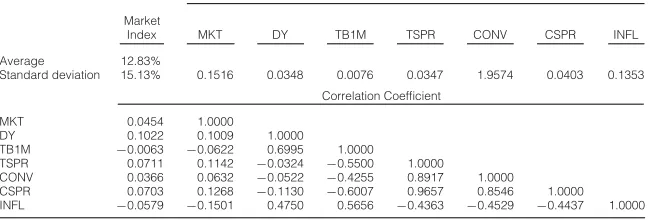
[image:14.441.60.388.246.356.2]Summary Statistics
Table 1 presents the summary statistics (averages, standard deviations, and correlations) for the market index and the 7 predictive instruments (lagged MKT, DY, TB1M, TSPR, CONV, CSPR, and INFL).
Predictive Instrument
Market
Index MKT DY TB1M TSPR CONV CSPR INFL
Average 12.83%
Standard deviation 15.13% 0.1516 0.0348 0.0076 0.0347 1.9574 0.0403 0.1353
Correlation Coefficient
MKT 0.0454 1.0000
DY 0.1022 0.1009 1.0000
TB1M −0.0063 −0.0622 0.6995 1.0000
TSPR 0.0711 0.1142 −0.0324 −0.5500 1.0000
CONV 0.0366 0.0632 −0.0522 −0.4255 0.8917 1.0000
CSPR 0.0703 0.1268 −0.1130 −0.6007 0.9657 0.8546 1.0000
INFL −0.0579 −0.1501 0.4750 0.5656 −0.4363 −0.4529 −0.4437 1.0000
There is relatively little persistence in market returns (with a 1st-order autocorrelation of only 0.05), which could be interpreted as evidence in support of weak-form efficiency. Consistent with standard business cycle theory, market returns are negatively correlated with interest rates and inflation. However, lagged CSPR is positively correlated with MKT, which seems counterintuitive at first but is consistent with the intuition developed in Fama and French (1989).
To begin with, we estimate the predictive regression (9) for each of the 3 sets of base assets, using each predictive instrument on its own in turn. We use monthly data from Jan. 1960 through 2004. The in-sample results are summarized in Table 2.
1. Single-Index Case
TABLE 2
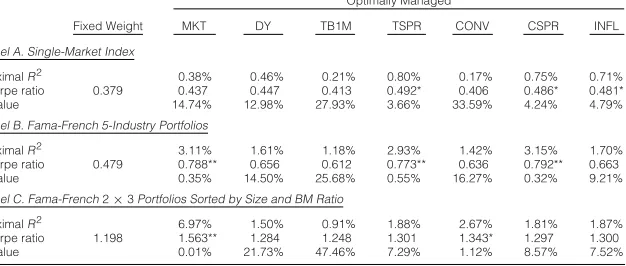
[image:15.441.69.382.158.291.2]In-Sample Results
Table 2 reports the in-sample estimation results of the predictive model, using different sets of base assets and each of the instruments (lagged MKT, DY, TB1M, TSPR, CONV, CSPR, and INFL) as predictive variables at a time. Panel A reports the results for a single-market index, while Panels B and C report the results using Fama and French’s 5-industry portfolios (available from Kenneth French’s Web site at http://mba.tuck.dartmouth.edu/pages/faculty/ken.french/data library.html), and the 2×3 portfolios sorted by size and BM ratio, respectively, as base assets. The (annualized) Sharpe ratios are computed as in Proposition 2, and thep-values are obtained from the standard Wald test for the slope coefficient in the predictive regression (4).
Optimally Managed
Fixed Weight MKT DY TB1M TSPR CONV CSPR INFL
Panel A. Single-Market Index
MaximalR2 0.38% 0.46% 0.21% 0.80% 0.17% 0.75% 0.71%
Sharpe ratio 0.379 0.437 0.447 0.413 0.492* 0.406 0.486* 0.481*
p-value 14.74% 12.98% 27.93% 3.66% 33.59% 4.24% 4.79%
Panel B. Fama-French 5-Industry Portfolios
MaximalR2 3.11% 1.61% 1.18% 2.93% 1.42% 3.15% 1.70%
Sharpe ratio 0.479 0.788** 0.656 0.612 0.773** 0.636 0.792** 0.663
p-value 0.35% 14.50% 25.68% 0.55% 16.27% 0.32% 9.21%
Panel C. Fama-French2×3Portfolios Sorted by Size and BM Ratio
MaximalR2 6.97% 1.50% 0.91% 1.88% 2.67% 1.81% 1.87%
Sharpe ratio 1.198 1.563** 1.284 1.248 1.301 1.343* 1.297 1.300
p-value 0.01% 21.73% 47.46% 7.29% 1.12% 8.57% 7.52%
for the mean-variance investor. Interestingly, although lagged DY has the highest correlation with market returns, it does not produce significant gains when used in a market-timing strategy (with a Sharpe ratio of 0.44, an insignificant increase with ap-value of 14.7%). This is consistent with the findings of, among others, Goyal and Welch (2003), who document that the predictive power of DY has diminished since the 1990s.
2. Multiple Risky Assets
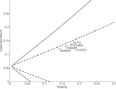
Panel B of Table 2 reports the analogous results using the 5-industry portfo-lios as base assets. The fixed-weight Sharpe ratio (0.48) is only marginally higher than in the single-index case, while the optimally managed Sharpe ratios now reach levels of almost 0.8. The regression coefficients (not reported in Table 2 to save space) are broadly consistent with those in the single-index case (with all instruments except TB1M and INFL having positive coefficients for all as-sets). The single exception is the health sector (HLTH), for which the sign of most coefficients is reversed, indicating the countercyclical nature of this sector. Again, even though the maximalR2range from only 1% to just over 3%, the effi-cient use of predictive information (in particular, lagged MKT, TSPR, and CSPR) considerably improves the investor’s risk-return trade-off (withp-values for the Wald test for predictability of 0.4%, 0.6% and 0.3%, respectively). The ranking of predictive instruments is broadly consistent with the single-index case, the only exceptions being lagged MKT (which is now highly significant) and INFL (which has lost some of its predictive power).
efficient in the fixed-weight sense, their average returns are about 10% lower than the return of a dynamically managed portfolio with similar risk!
[image:16.441.100.340.436.623.2]Panel C of Table 2 finally reports the analogous results using the 2×3 size and BM portfolios as base assets. Again, the coefficients of the predictive re-gression (not reported in Table 2 to save space) are broadly consistent with the single-index case (with all instruments except TB1M and INFL having positive coefficients for all assets). However, unlike in the case of the industry portfo-lios, there is a clear pattern in the magnitude of the coefficients: For almost all predictors, the coefficients on the small-cap portfolios are considerably larger in absolute value than those for the large-cap portfolios. This indicates that returns on small stocks are more predictable than those of large stocks. For the size and BM portfolios, even the fixed-weight Sharpe ratio now more than triples (1.20). This is because when the investor is allowed to select stocks on the basis of size and BM ratio, even a static portfolio can take advantage of the well-documented size and value premia (Fama and French (1992)). However, even though the ab-solute levels are very different for the 2 asset sets, therelativeincrease in Sharpe ratio due to the optimal use of predictive information is remarkably similar. The best-performing predictors are still lagged MKT, TSPR, CONV, CSPR, and INFL, although the ranking has changed slightly (with CONV now playing a significant role, while TSPR and CSPR have lost some of their power).
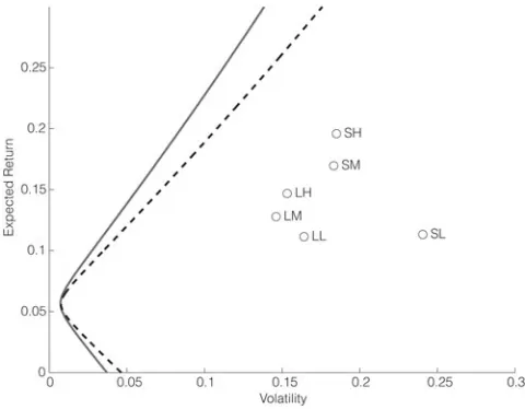
Figure 2 shows the efficient frontiers, with (solid line) and without (dashed line) the optimal use of predictive information (here, TSPR, CONV, and INFL are used as instruments). In contrast to the industry portfolios, the size and BM portfolios themselves are far from being even fixed-weight efficient. This is be-cause even a static portfolio can exploit the size and value premium by trading the
FIGURE 2
Efficient Frontiers
spread between small and large stocks, and value and growth stocks. However, the optimal use of predictability still yields substantial economic gains, achieving almost 5% more return at 10% volatility than the efficient fixed-weight portfolio.
C. Portfolio Performance
While the preceding sections documented the potentialgains from return predictability, in this section we focus on analyzing the ex post performance of the dynamically managed strategies that exploit this predictability. To do this, we estimate the predictive model (9) and use the estimated coefficients to con-struct dynamically efficient portfolio strategies as in Proposition 4. We then com-pute the returns on these strategies and evaluate their performance using a variety of industry-standard performance measures. The results are reported in Table 3 (although we tested 3 types of strategies—maximum-return, minimum-variance, and maximum-utility—we only report the performance figures for the minimum-variance portfolios to save space, but the results for the other strategies are very similar).
TABLE 3
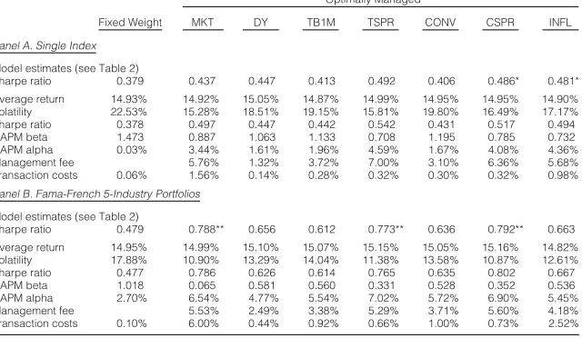
[image:17.441.63.383.354.540.2]Portfolio Performance
Table 3 reports the ex post performance of fixed-weight and dynamically managed portfolios. In Panel A the single-market index is used as base asset, while Panel B reports the results for the 5-industry portfolios. The predictive model is estimated for each set of assets and each of the predictive instruments. Based on the parameter estimates, efficient minimum-variance portfolios (with a target mean of 15%) are constructed as in Proposition 4, and their performance is evaluated over the entire sample period. Return, volatility, Sharpe ratio, and alpha are annualized.
Optimally Managed
Fixed Weight MKT DY TB1M TSPR CONV CSPR INFL
Panel A. Single Index
Model estimates (see Table 2)
Sharpe ratio 0.379 0.437 0.447 0.413 0.492 0.406 0.486* 0.481*
Average return 14.93% 14.92% 15.05% 14.87% 14.99% 14.95% 14.95% 14.90%
Volatility 22.53% 15.28% 18.51% 19.15% 15.81% 19.80% 16.49% 17.17%
Sharpe ratio 0.378 0.497 0.447 0.442 0.542 0.431 0.517 0.494
CAPM beta 1.473 0.887 1.063 1.133 0.708 1.195 0.785 0.732
CAPM alpha 0.03% 3.44% 1.61% 1.96% 4.59% 1.67% 4.08% 4.36%
Management fee 5.76% 1.32% 3.72% 7.00% 3.10% 6.36% 5.68%
Transaction costs 0.06% 1.56% 0.14% 0.28% 0.32% 0.30% 0.32% 0.98%
Panel B. Fama-French 5-Industry Portfolios
Model estimates (see Table 2)
Sharpe ratio 0.479 0.788** 0.656 0.612 0.773** 0.636 0.792** 0.663
Average return 14.95% 14.99% 15.10% 15.07% 15.15% 15.05% 15.16% 14.82%
Volatility 17.88% 10.90% 13.29% 14.04% 11.38% 13.58% 10.87% 12.61%
Sharpe ratio 0.477 0.786 0.626 0.614 0.765 0.635 0.802 0.667
CAPM beta 1.018 0.065 0.581 0.560 0.331 0.528 0.352 0.536
CAPM alpha 2.70% 6.54% 4.77% 5.54% 7.02% 5.72% 6.90% 5.45%
Management fee 5.53% 2.49% 3.38% 5.29% 3.71% 5.60% 4.18%
Transaction costs 0.10% 6.00% 0.44% 0.92% 0.66% 1.00% 0.73% 2.52%
1. Single Risky Asset Case
match the theoretically predicted ones and exceed the latter for “good” predictors (in the single-index case, TSPR, CSPR, and INFL). The minimum-variance strate-gies match their target mean (15%) almost perfectly, while the volatility of the maximum-return strategies (not reported in Table 3) often falls below the target (15%) (in particular for “good” predictors). The dynamically managed strategies clearly outperform their fixed-weight efficient counterparts (e.g., the maximum-return strategy using TSPR achieves almost 2% more maximum-return at almost 2.5% less volatility, while the corresponding minimum-variance strategy reduces volatility from 23% to 16% without sacrificing return).
The quality of the predictive instrument is reflected in the strategy’s beta relative to the market index: While strategies based on “bad” predictors effec-tively track the index (with betas close to 1.0), “good” predictors allow the strat-egy to successfully “decouple” itself from the index (with betas of 0.60, 0.66, and 0.61 for TSPR, CSPR, and INFL, respectively). In other words, the predictive information allows the strategy to “time the market,” dynamically shifting funds between the index portfolio and the risk-free asset.
While the efficient fixed-weight strategies fail to “beat the market” (with alphas of about 0.03%), the dynamically managed portfolios outperform the market benchmark by a wide margin (with alphas of up to 4.5% per annum). Interestingly, the minimum-variance strategies achieve higher alphas than their maximum-return counterparts. This is probably due to the fact that the former have lower tracking errors.
2. Multiple Risky Assets
Panel B of Table 3 reports the analogous results using the 5-industry port-folio as base assets. The results are qualitatively very similar to the single-index case: The ex post performance matches the theoretically predicted one closely. Being able to dynamically allocate funds across different assets allows portfo-lio managers to “decouple” their strategies even more from the index (with betas as low as 0.3). Although the fixed-weight efficient portfolios now outperform the benchmark (with alphas of 2.3% and 2.7%), the dynamically managed strategies achieve in-sample alphas in excess of 9% per annum! In contrast to the market-timing strategies considered in the preceding section, the alphas of maximum-return strategies are now consistently higher than those of the corresponding minimum-variance strategies. One possible explanation is that in the market-timing case, maximum-return strategies are constrained to track a given target volatility. Overall, the increase in performance compared to Panel A of Table 3 indicates that return predictability is not just about “timing the business cycle,” but that dynamic asset allocation plays just as important a role.
FIGURE 3
Minimum-Variance and Maximum-Return Portfolios
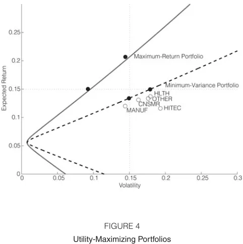
[image:19.441.99.340.137.379.2]Figure 3 shows the ex post performance (average return and volatility) of the fixed-weight and optimally managed minimum-variance and maximum-return portfolios, respectively, relative to the fixed-weight (dashed line) and dynamically optimal (solid line) ex ante efficient frontiers. The base assets are the 5-industry portfolios (shown as circles), and the instruments are TSPR, CSPR, and INFL.
FIGURE 4
[image:19.441.100.338.424.610.2]Utility-Maximizing Portfolios
less risk-averse investors stand to gain more from predictability (see also next section).
D. Economic Value
To assess the economic value of predictability, we estimate the “management fee” that a risk-averse investor would be willing to pay for the superior strat-egy (Fleming et al. (2001)). The results (selected figures are reported in Tables 3 and 4) are consistent with our earlier findings, with “good” predictors support-ing management premia from 2.50% to more than 6% per annum (for these figures, we used a moderate risk-aversion coefficient of 5). While for maximum-return strategies, the management premium is only very slightly decreasing in risk aversion (ranging from 4.5% to 4.2%, using TSPR as predictor), the premium for minimum-variance strategies strongly increases with the investor’s risk aversion (ranging from 1.2%, for a very low risk-aversion coefficient of 1, to 10.9%, for a coefficient of 10). This makes sense, as the maximum-return strategy is con-strained to track a fixed volatility target, so that its utility is largely unaffected by the risk-aversion coefficient. For the utility-maximizing strategies (see Table 4), the management premium strongly decreases with increasing risk aversion. This is due to the fact that risk-tolerant investors will choose a portfolio “further up” the efficient frontier, where the “spread” between fixed-weight and optimally man-aged portfolios is wider (see also Figure 4).
TABLE 4
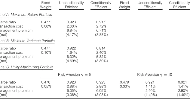
[image:20.441.66.382.400.567.2]Comparison of Unconditionally and Conditionally Efficient Strategies
Table 4 compares the performance of fixed-weight, unconditionally and conditionally efficient maximum-return, minimum-variance, and maximum-utility portfolios, respectively. The rows labeled “(net)” refer to the management premium that an investor would pay after transaction costs have been deducted. The base assets are the 5-industry portfolios, and the instruments are TSPR, CSPR, and INFL. All figures are annualized.
Fixed Unconditionally Conditionally Fixed Unconditionally Conditionally
Weight Efficient Efficient Weight Efficient Efficient
Panel A. Maximum-Return Portfolio
Sharpe ratio 0.477 0.923 0.917
Transaction cost 0.08% 2.60% 2.72%
Management premium 6.84% 6.71%
(net) (4.17%) (3.88%)
Panel B. Minimum-Variance Portfolio
Sharpe ratio 0.477 0.922 0.814
Transaction cost 0.10% 1.64% 2.40%
Management premium 6.32% 5.82%
(net) (4.69%) (3.39%)
Panel C. Utility-Maximizing Portfolio
Risk Aversionγ=5 Risk Aversionγ=10
Sharpe ratio 0.478 0.923 0.923 0.479 0.921 0.921
Transaction cost 0.05% 2.88% 2.88% 0.03% 1.41% 1.41%
Management premium 6.05% 6.05% 2.90% 2.90%
(net) (3.08%) (3.08%) (1.49%) (1.49%)
instruments. However, we find that the performance of this model does not even come close to that of a simple linear predictive model.
E. Transaction Costs
To assess the practicability of our strategies, we estimate the total transaction costs11incurred each period as a fraction of portfolio value, for both the in- and out-of-sample (see later) applications. Overall, transaction costs destroy only a very small fraction of the portfolios’ performance (ranging from 0.10% to 0.30% per annum for market-timing strategies, and 0.50% to 1.00% per annum in the multiasset cases; see Table 5). This still leaves net management premia of up to 6%. Interestingly, the relation between the predictive ability of an instrument and the cost of the corresponding strategy is not always monotonic: While strategies based on “bad” predictors (e.g., DY or TB1M) are generally cheaper (because the strategy has no meaningful signal to respond to), the cost of “good” strategies varies substantially across instruments. Strategies based on INFL or lagged MKT are 3–5 times more expensive than those based on term structure instruments (i.e., TSPR, CONV, and CSPR). In fact, in the multiasset cases, the transaction costs of strategies based on lagged MKT and INFL wipe out the entire manage-ment fee, making the strategy unattractive to a moderately risk-averse investor. The transaction cost effects of the different instruments likely reflect their relative
TABLE 5
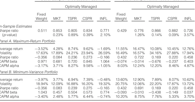
[image:21.441.61.382.409.577.2]Out-of-Sample Portfolio Performance (5-industry portfolios)
Table 5 reports theout-of-sampleperformance of fixed-weight and dynamically managed maximum-return and minimum-variance portfolios, respectively. The model is estimated for the in-sample period, using the 5-industry portfolios as base asset and each of the instruments as predictor variables. Based on the parameter estimates, efficient portfolios are con-structed as in Proposition 4, and their performance evaluated over the out-of-sample period. Return, volatility, Sharpe ratio, and alpha are annualized.
Out-of-Sample Period 2000:01–2004:12 Out-of-Sample Period 1995:01–2004:12
Optimally Managed Optimally Managed
Fixed Fixed
Weight MKT TSPR CSPR INFL Weight MKT TSPR CSPR INFL
In-Sample Estimates
Sharpe ratio 0.511 0.853 0.805 0.834 0.771 0.429 0.776 0.866 0.882 0.726
(p-value) 0.23% 0.89% 0.39% 2.10% 1.26% 0.14% 0.09% 3.57%
Panel A. Maximum-Return Portfolio
Average return −3.52% 4.28% 8.74% 9.62% −1.69% 11.55% 16.47% 10.08% 10.45% 12.76% Volatility 17.63% 17.89% 24.21% 23.94% 26.59% 16.49% 16.57% 34.16% 27.88% 17.94% Sharpe ratio −0.356 0.084 0.236 0.273 −0.166 0.432 0.722 0.169 0.220 0.458 CAPM beta 0.971 0.681 0.720 0.845 1.064 −0.074 −0.014 −0.676 −0.237 0.403 CAPM alpha −3.17% 3.71% 8.27% 9.58% −1.05% 8.03% 12.24% 12.20% 8.46% 4.87%
Panel B. Minimum-Variance Portfolio
Average return −3.97% 3.77% 6.94% 7.39% −0.48% 13.60% 12.90% 7.89% 8.07% 10.62% Volatility 18.94% 12.09% 16.88% 16.20% 19.32% 20.75% 12.06% 22.20% 17.87% 13.72% Sharpe ratio −0.356 0.083 0.239 0.275 −0.165 0.432 0.691 0.169 0.220 0.458 CAPM beta 1.043 0.457 0.504 0.573 0.774 −0.093 −0.010 −0.438 −0.149 0.037
CAPM alpha −3.40% 2.48% 5.77% 6.44% −0.74% 10.20% 8.75% 7.76% 5.33% 3.70%
11We ignore fixed costs and assume transaction costs of 20 basis points (bp) (as a percentage of
persistence. Lagged MKT and INFL deliver more volatile fitted expected returns, and thus more trading, than the persistent interest rate variables.
F. Comparison with Conditionally Efficient Strategies
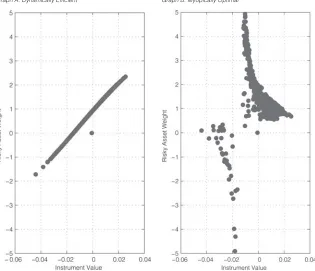
When we compare the performance of our dynamically efficient strategies with that of their corresponding conditionally efficient counterparts (selected results reported in Table 4), three consistent patterns emerge: First, condition-ally efficient strategies never outperform their dynamiccondition-ally efficient counterparts, and in many cases they significantly underperform. Second, dynamically effi-cient strategies are consistently cheaper to run, the difference in costs being most pronounced (see Table 4) for minimum-variance strategies. Third, conditionally optimal strategies are much more sensitive to short-sale constraints, as they of-ten require extreme shifts between long and short positions in excess of 200% (see Figure 5). In fact, we find that in contrast to our dynamically efficient strate-gies, conditionally efficient strategies often improve in performance when short-sale constraints are imposed. This is in line with the findings of Frost and Savarino (1988) and Jagannathan and Ma (2003).
FIGURE 5
[image:22.441.64.379.351.622.2]Efficient Portfolio Weights
Figure 5 shows the efficient weights on the risky asset as a function of (the optimal linear combination of) the predictive instruments, for the case of a single-market index as risky asset. Graph A shows the weights of the unconditionally efficient (dynamically efficient) strategy, while Graph B shows the weights for the conditionally efficient (myopically optimal) strategy. The predictive instruments are TSPR, CSPR, and INFL.
These effects are due to the fact that dynamically efficient strategies display a much more “conservative” response to extreme changes in the predictive instru-ment (see also Section II.E), a fact also observed by Ferson and Siegel (2001). For example, Figure 5 shows the weights of the 2 types of strategies on the single risky index, as a function of (the optimal linear combination of) the predictive instruments. The figure shows that even for very small changes in the predictive instruments, the weights of the conditionally optimal strategy (Graph B) often require sudden changes between extreme long and short positions.
G. Out-of-Sample Performance
To assess the out-of-sample performance of our strategies, we conduct 3 experiments: First, we estimate the predictive model using a subsample of the original 1960–2004 data, and then we evaluate the performance of the resulting strategies over the entire remaining sample period. As cutoff points for the out-of-sample periods, we choose Jan. 1995 (the beginning of the “dot.com” boom), and 2000 (the beginning of the collapse of the bubble). Second, we run “rolling window” experiments, in which the model is estimated over a 5- or 10-year pe-riod, the resulting strategy is run over the 12 months following the estimation period, and then the estimation window is rolled forward by 1 year. Finally, we estimate the performance of our strategies over the 2005–2009 period (which includes the “credit crunch” and subsequent economic downturn), using data that has not been utilized in any of our in-sample estimations.
Table 5 presents the out-of-sample performance of several dynamically effi-cient strategies in the 2 chosen out-of-sample periods, using the 5-industry portfo-lios as base assets. Of course, the out-of-sample performance, in particular, in the 2000–2004 period case, does not match that predicted by the estimation (because the model was estimated over a bull run, but the strategy was run through a bear market). However, the performancerelativeto MKT (or the efficient fixed-weight strategy) is largely consistent with our in-sample results. Specifically, we find that strategies based on TSPR and CSPR outperform the market index by a margin of 6%–12% in both cases. While the term structure variables generate good perfor-mance in both out-of-sample periods, the results for other predictors are mixed: While lagged MKT perform well in the “dot.com” boom (1995–2004), they do not add much value during the collapse of the bubble (2000–2004). Conversely, strate-gies based on INFL in fact underperform during the bear market, while showing moderate performance during the rise of the bubble. In other words, our findings suggest that the level and shape of the term structure is the only information that is consistently useful in predicting stock returns, while other variables do well in bull markets but fail in bear markets or vice versa.
FIGURE 6
Out-of-Sample Portfolio Performance (5-industry portfolios)
Graph A of Figure 6 shows theout-of-sampleperformance (cumulative return) of the fixed-weight (dashed line) and op-timally managed (bold-faced line) maximum-return portfolio, relative to the performance of the market index (light-weight line). The model is estimated using data until Dec. 1999, and the strategy is evaluated in the out-of-sample period from 2000 through 2004. Graph B shows the time series of the instruments used: TSPR (“+”) and CONV (“◦”).
Graph A. Cumulative Return
Graph B. Predictive Instruments
1. Rolling Window
Second, we run “rolling window” experiments, in which the model is esti-mated over a 5- or 10-year period, the resulting strategy is run over the 12 months following the estimation period, and then the estimation window is rolled for-ward by 1 year. We find that the strategies obtained this way perform much worse than in the simple out-of-sample experiments. We attribute this to the fact that dynamically efficient strategies are designed to be optimal with respect to long-run unconditional moments. Reestimating the model each year and allowing the strategy to run only for 1 year at a time is contrary to this philosophy, as the long-run mean cannot be attained over such short periods, while the risk is amplified due to the lack of time aggregation (because the strategy “thinks” that there is only 1 period to respond to the information, it tends to “overreact”).
2. Performance after 2004
We estimate the predictive model using the original 1960–2004 data, then formed optimal dynamic portfolio strategies on the basis of the estimated model coefficients and assessed the performance of these strategies in the period after 2004.
remains strong. For example, using the 4 predictive variables that had shown the strongest performance in the in-sample estimation (TSPR, CONV, CSPR, and INFL), we found that the single-index market-timing strategy achieved a Sharpe ratio of 1.3 from 2005 through 2007, compared with only 0.74 for the fixed-weight strategy. Interestingly however, the out-of-sample performance of both the fixed-weight and the dynamically optimal strategy exceeded the in-sample predictions (which were 0.48 and 0.85, respectively).
While the fixed-weight strategy underperformed relative to the market in-dex (with a negative alpha), the dynamically managed strategies achieved alphas of between 5% (for the maximum-return strategy) and 7.4% (for the minimum-variance strategy). Even after the deduction of transaction costs, risk-averse in-vestors would still be willing to pay an annual fee of about 150–400 bp for this strategy. Moreover, the unconditionally efficient strategies beat their conditionally efficient counterparts by a wide margin in this period; the latter achieved lower Sharpe ratios while experiencing much higher volatility in portfolio weights, resulting in higher transaction costs and a negative management fee (i.e., investors would rather “burn money” than invest in these strategies).
On the other hand, strategies based on the 5-industry portfolios do not sustain their superior performance in the 2005–2007 period. In fact, while the fixed-weight strategies in this case still achieve a respectable Sharpe ratio and a marginally positive alpha, all managed strategies (both unconditionally and conditionally efficient, with or without short-sale constraints) underperform. This suggests that, in the period after 2004, market timing still worked (i.e., the predic-tive variables told investors when to “get out” of the market), but the predicpredic-tive relationship between the instruments and optimal asset allocation seems to be broken.
An interesting observation is that when we remove CSPR from the set of pre-dictive variables, the performance of our strategies increased dramatically (from underperforming the market to achieving a Sharpe ratio of almost 1.0 and earn-ing a 250-bp management fee). This suggests that the predictive ability of the
averagecredit spread was not sufficient to select among different industries in the post-2004 period. This observation, together with the fact that market-timing strategies still worked well using CSPR, seems to indicate that there were a lot of idiosyncratic (sector-specific) movements during this period that the average spread was not able to discern.
In our final experiment, we keep the in-sample period (1960–2004) but ex-tend the out-of-sample period all the way to June 2009. In this case, we have to admit that none of our strategies managed to avoid the losses incurred by the mar-ket. In fact, most of the dynamically managed strategies even underperformed during the final 18 months (i.e., during the “credit crunch” and the subsequent economic meltdown). This (quite plausibly, given recent events) suggests a regime shift in the relation between predictive instruments and market returns.
H. Robustness
simulation experiments under the null hypothesis and the alternative, respectively. In both cases, we first fit a (vector) AR(1) model to the original time series of instrument(s), and then simulate 100,000 new time series by resampling from the residuals of this estimation and then reconstructing the instrument values using the AR(1) coefficients.
1. Simulation under the Null Hypothesis
[image:26.441.61.379.421.582.2]To simulate the corresponding time series of asset returns under the null hy-pothesis (of no predictability), we draw independent samples from the uncon-ditional empirical distribution of asset returns. In other words, this procedure assumes that the time series of asset returns is i.i.d. (with the marginals given by the empirical distribution of the original data) and independent of the instru-ments, thus modeling the null hypothesis of no predictability. For each of the 100,000 simulated time series of returns and instruments, we then reestimate the predictive model (9) and compute the implied Sharpe ratios from equation (3).
Figure 7 shows the result of the bootstrap simulation for the single-index model, using TSPR, CONV, and CSPR as predictors. Graph A plots the opti-mally managed (vertical axis) against the fixed-weight (horizontal axis) annual-ized Sharpe ratios, estimated from the simulated time series.12 The dashed lines show the Sharpe ratios derived from the original model estimation (0.379 fixed-weight and 0.557 optimal). The empirical p-value of 6.13% obtained from
FIGURE 7
Bootstrap (null hypothesis)
Figure 7 shows the result of the bootstrap experiment (see Section III.H) under the null hypothesis. Graph A plots the optimally managed (vertical axis) against the fixed-weight (horizontal axis) annualized Sharpe ratios, estimated from the simulated time series of asset returns and instruments. The solid lines show the 95% confidence interval for the test statistic Ω. Also shown are the Sharpe ratios estimated from the original data (dashed lines). Graph B plots the theoretical (asymp-toticχ2) distributions of the Wald test for the slope coefficient in the predictive regression (4), and the empirical distribution obtained from the bootstrap simulation.
Graph A. Bootstrap Graph B. Empirical and Theoretical(χ2)Distribution
12For clarity of the graphical representation, we only plot the first 10,000 samples, although
the simulation closely matches the theoretical one of 6.21% (derived from the asymptoticχ2distribution of the test statistic, see Proposition 3).
Graph B of Figure 7 shows the empirical distribution of the test statistic Ω, obtained from the simulation, compared with theχ2 distribution of the Wald test statistic of the slope coefficient in the predictive regression. Although the empirical distribution displays very slight excess skewness (1.69 compared with the theoretical 1.63) and kurtosis (7.52 compared with 7.50), the match is very close. The bootstrap thus confirms our theoretical results, and moreover shows that neither nonnormality nor finite-sample problems significantly affect our em-pirical findings. We conduct the same experiment for all other combinations of assets and/or instruments and find in all cases a similarly close match between theoretical and empirical distribution.
2. Simulation under the Alternative
To construct the corresponding experiment under the alternative, we first es-timate the predictive model (9) using the original data and then construct 100,000 simulated time series by simultaneously resampling the residuals of the AR(1) model for the instruments and the predictive model for asset returns. In other words, the originally estimated predictive relation between lagged instruments and asset returns is assumed to be the true data-generating process for this simu-lation, thus modeling the alternative to the null hypothesis of no predictability.
The results for the single-index model, using TSPR, CONV, and CSPR as predictors, are shown in Figure 8. To match the empirical distribution of the test statistic Ω under the alternative, we fit a noncentral χ2 distribution, with the
FIGURE 8
[image:27.441.57.378.470.618.2]Bootstrap (alternative)
Figure 8 shows the result of the bootstrap experiment (see Section III.H) under the alternative. Graph A plots the optimally managed (vertical axis) against the fixed-weight (horizontal axis) annualized Sharpe ratios, estimated from the simulated time series of asset returns and instruments. The solid lines show the 95% confidence interval for the test statisticΩ. Also shown are the Sharpe ratios estimated from the original data (dashed lines). Graph B plots the theoretical (asymptotic χ2) distributions of the Wald test for the slope coefficient in the predictive regression (4), and the empirical distribution obtained from the bootstrap simulation.