Adapting the variational auto encoder for datasets with large amounts of missing values

Adapting the variational auto encoder for datasets with large amounts

of missing values.

Raoul Fasel

Abstract— This research provides an adaptation to the Vari-ational Auto Encoder(VAE) aimed at handling missing values. This adaptation comes in the form of a modified loss function. different VAE configurations are trained and evaluated on real-world data. These configurations include, next to the normal and modified loss functions, different beta parameters and usage of beta annealing. Practical implementations of the VAE or parts of it include dimensionality reduction and classification using network pretraining or a data preprocessor. While the modified loss function has a big influence on the VAE during training and reconstructing tasks, it does not have any influence on the performance of classification when either used as a data preprocessor or as a pretrained network. Lower beta values are preferred for reconstruction tasks and classification using a pretrained network. Higher beta values are preferred when using the VAE as a data preprocessor for classification. Annealing has shown to have no usable influence in research.

I. INTRODUCTION

Machine learning has become a very popular research topic in the past decades. Thanks to this, artificial intelligence have been outperforming humans in very complex tasks [1]. While very impressive, this research is often accompanied by an abundance of high-quality data or an ability to collect high-quality data. However, not every data source in the real world can be considered high quality. One of the problems with real-world datasets is that they contain a lot of missing values [2][3]. The reasons for missing values can vary, for example missing values because of errors during acquisition or addition of new variables to an existing dataset. Further-more, data gathering is often done by collecting everything that is available without knowing how much information is gained for solving the required task. This leads to data with many dimensions that are hard to deal with [4]. Another smaller problem is imbalanced data in which not every class is equally represented.

Traditionally, imputation during prepossessing was used to fill in the missing values. It is also possible to use algorithms that can deal with missing values, for example, neural networks have proven to be robust when dealing with missing values[2] [5]. An easy method for dealing with the number of dimensions of your data is selecting features that are most important for the task at hand and only using these features leading to some information loss. A more universal technique would be using some kind of dimensionality reduction technique like principal component analysis (PCA) [6]. PCA minimizes information loss. Class

1_{R. Fasel is with Faculty of Electrical Engineering, Mathematics and}

Computer Science, University of Twente, 7500 AE Enschede, The Nether-landsr.fasel at student.utwente.nl

imbalance problems are often mitigated by simple class weighting or over- and under-sampling [7].

We propose a novel loss function that allows a Variational Autoencoder (VAE) [8] to not learn from missing values and only learn from the data that is actually available. The VAE is able to reduce highly dimensional data that contain lots of missing values, making it suitable for usage on real-world data. Practical usage examples of the VAE are also provided and evaluated. These examples include predicting consumer buying patterns by using the VAE as a pre-trained part of a neural network trained for classification and by using the VAE as a dimensionality reduction data pre-possessor that can be used like PCA on any classifier. Next to the methods based on the VAE a semi-supervised Generative Adversarial Network (SGAN)[9][10], random forest[11] and boosted tree[12] were also implemented and evaluated on the unmodified dataset. These were used as a baseline for comparisons. Both training and evaluating were done on a real-world dataset.

A. Dataset

Such a real-world dataset was provided for this research by an external company called Centraal Beheer (CB). CB is one of the bigger insurance companies in the Netherlands. The interests of CB are as follows: Predicting buying patterns of customers using Neural Networks and dimensionality reduction. Because of the amount of data and the number of variables, CB would like this research to include dimension-ality reduction techniques. Secondary interest of CB includes data generation and in-depth model explanation.

The dataset consists of almost 600.000 unique customers. Every customer has up to 5000 variables in this dataset. The number of variables per customer is highly variable however. The dataset is very sparse, with lots of missing values. These missing values may not be available because it has not been recorded as of now, could not be recorded or because it is dependent on another variable. Dependency information, however, is not available.

highly imbalanced, with only 6000 customers belonging to the class that has bought anything after the email campaign. Four distinct datatype variations are identifiable, these include binary data, categorical data, continuous numerical data and time data. The numerical data contains arbitrary numbers, for example, money claimed in the last month. The time data contains timestamps of events, for example, the last visit on a website. An example of a binary variable would be whether the user is the owner of a car. The categorical data contains codes, for example the variableINSURANCETYPE can contain PREM or STAN standing for a premium or standard insurance respectively.

II. RELATED WORK

Unsupervised pre-training is a technique that can be used to improve the performance of deep learning. According to Erhan et al. [13] unsupervised pre-training causes networks to generalize consistently better compared to randomly ini-tialized networks. Unsupervised pre-training works by letting a neural network learn the intricate dependencies between parameters without using class labels that could influence these dependencies. An example of a network that allows for unsupervised pre-training is an autoencoder [14]. An autoencoder is a neural network that learns a set of latent variables by itself by encoding examples to a latent space and then decoding from a latent space while minimizing the information loss between the original data point and its decoded counterpart. The encoding and decoding are done in one single pass. The benefit of an autoencoder is the fact that the decoding and encoding parts can be used as pre-trained networks in generative and discriminating tasks. The encoder could also be used as a compression system on its own. However, this compression is rarely lossless. The autoencoder will select the latent variables best suited for reconstruction. Whether these latent variables are also best suited for classification remains to be seen.

Beaulieu-Jones et al. [15] provide an autoencoder with a modified loss function that handles missing values. The modified loss function does not calculate loss over variables within a datapoint that are missing. It does this by adding extra binary variables to each original variable that track if the original variable was missing or not. Beaulieu-Jones et al. concluded that this technique is a robust alternative compared to traditionally popular imputation techniques. These techniques include imputation by mean averaging, me-dian averaging or K nearest neighbor. Beaulieu-Jones et al. does only explore the reconstruction imputation performance and does not experiment with the usability of the latent dimension.

Ennett et al. [5] show that Neural networks can work with missing values without any modification by simply replacing the missing values with zeros. This way the input neurons are not activated during classification. Different versions of artificially created data with missings were made and compared to a constant predictor baseline. While the goal of the research was to find a breaking point of the neural network all versions performed better than the baseline.

Kingma et al. [8] provide an adaptation of the Autoencoder network called the Variational Autoencoder (VAE). The VAE inherits the basic Autoencoder architecture but extends it with a Variational Bayes approach. In a VAE the encoder does not simply output a vector of latent variables but two vectors, one that contains the means and one that contains the standard deviations of the latent variables. These vectors are then used to sample the encodings. This means that for the same input the encoding can be slightly different on every pass while keeping the means and standard deviations the same. An extra cost function based on the Kullback Leiber divergence [16] is added to the loss function in order to penalize distributions that drift away from the other distributions during training. The complete loss function can be simplified to the following formula:

L=R+K (1)

WhereR is the reconstruction loss overall input and output variables, for example, MSE andK is the Kullback Leiber divergence. Thanks to all this the VAE makes it hard for the autoencoder to ”memorize” specific cases in the latent space, which is a possibility when only having the reconstruction loss like in an AE. The VAE is suited for use on big data because it allows efficient training using very small batch sizes or even single data points according to Kingma et al. Like an autoencoder the decoder can be used as a pre-trained part in a generative model and the encoder can be used as a pre-trained part of a discriminating model.

The KL divergence term used in the VAE can be controlled as first proposed by Higgins et al. [17]. Higgins et al. control the KL term by introducing a simple hyper-parameterβand finally conclude that aβ >1can lead to more disentangled learning. The bestβcould be found using a basic grid search method. Thisβ however could also be increased from 0 to 1 during training. This was discovered by Bownman et al. [18]. Bownman calls this KL cost annealing and was discovered to improve the training of the network. Intuitively KL cost annealing works by first letting the network learn as much as possible without any constraint because the β is zero. Equation 1 can be expanded in to the following simplified formula:

loss=R+β∗K (2)

When the β increases it slowly forces to generalize better like a standard VAE. According to the results of Bownman and Higgins it would be very interesting to experiment with a slowly increasingβ and with a β >1.

calculate a cost on every layer between the ”clean” encoder and decoder. This cost is used in the loss function that consists of the weighted mean of every layer costs added to the cross-entropy calculated between the true label and the label predicted by the corrupted encoder. The setup is rather complex but proven [21] and does not require pre-training.

The Generative Adversarial Nets(GAN) framework was first proposed by Goodfellow et al. [22]. This framework trains two models at the same time in an unsupervised adversarial manner. The discriminative model has the result from the generative model as input. The generative model uses random data from a normalized This can be explained by seeing the two models as players in a mini-max two-player game. One two-player tries to ”fake” examples while the other tries to recognize the fakes. The discriminative model has the result from the generative model and known ”real” data as input. The generative model uses random data from a normalized and predefined latent space. The discriminator can be pre-trained using known examples to avoid a generator that is too good which will lead to the discriminator not learning anything.

A GAN can be adapted for classification by adding an extra output [9], creating a semi-supervised GAN (SGAN). In an SGAN the discriminator is adapted into a combined discriminator and classifier. Instead of a single sigmoid output unit, the output consists of multiple outputs with a Softmax activation. One output denoting real classes, replacing the sigmoid output in a GAN, and the addition of one softmax output for every class in the dataset. Ac-cording to the results of the initial papers [10] [9] these improvements benefit both the generative performance and the classification performance when compared to a GAN and a more traditional supervised Neural Network. The combination of generative and classification within a single network and the ability of semi-supervised learning makes this type of network highly suited for the interests of CB. This single network can full fill both the generative and classification requirements while keeping the implementation time and learning time lower by only needing one model. A disadvantage, however, is the fact that is network is trained on a labeled dataset, thus possibly influencing the resulting generator.

Evaluating generative models is different from classifica-tion models because no ground truth exists. Instead, genera-tive models are evaluated by the likelihood of the generated data belonging to the target datatype. Often evaluation is done by human assessment of generated samples when cal-culating likelihood is impossible or unpractical. For example, GAN models trained on visual data can be evaluated by humans [10]. However visual assessment of samples does not always correlate with likelihood according to Theis et al. [23]. Even though Theis et al. denote the use of visual assessment as generally a poor evaluation technique, they do note that using visual assessment evaluation for the purpose of creating purely visual pleasant images is valid. Theis et al. conclude that there is no one size fits all solution to model evaluation and that human assessment can only be used as

a measure in the specific assessment context and not as a general model performance metric.

The dataset used in this research is not visual however the same core concepts could be used. For example, when a human assesses a generated human head the human will look for human head shape and will consider the image as wrong if he finds a triangle shape with eyes. A triangular head can simply not exists, in other words, some rules could be defined that can be used by the assessor. The same is true for this data set. Especially within the dependency of some of the variables. For example, a customer with age below 18 and a car insurance can simply not exist. These rules could be tested automatically. However when going back to the results of Theis et al. high results on these automated test do only prove that the generated samples will be assessed as real by human annotators. It will not prove that the generator was able to capture the distribution of the original dataset. Moreover, no validated set of such rules is currently available so a working implementation of this system cannot even be implemented.

Because the dataset is highly imbalanced and because the important label is the least represented in the dataset. It is important to make a classifier in such a way that it takes the importance of the label into account. This is called Cost-Sensitive Learning [7]. These techniques are often applied to medical classification problems where finding true positives are very important compared to other metrics, for example, the accuracy of the classifier as a whole. One technique to apply Cost-Sensitive Learning is Class Weighting [24] where the classes get a weight that represents the importance of the class. This weight is used to alter the miss-classification cost. Different re-sampling techniques can also be used to counter this imbalance problem. For example, oversampling of the minority class using adaptive synthetic sampling (ADASYN) [25] or Synthetic Minority Over-sampling Tech-nique (SMOTE) [26]. Both of these techTech-niques generate synthetic examples that fit in the distribution of the original class. Another example is undersampling which as the name suggests decreases the number datapoints in the majority class while also keeping the distribution of these data points the same as the original.

III. METHODSAND MODELS

This section describes the methods and models used in this research. This section is divided into subsections. The first one III-A describes the pre-processing done to the data. This pre-processing was used for the models described in the later subsections. The implementation of these models, including prepossessing functions can be found on GitLab [27]. The implementation was done using the Python language together with some well-established Python libraries including but not limited toKeras[28] and the SciPytoolkit [29]

A. Data preparation and missing values

prepa-rations were made to allow the models to handle missing values. All missing values were encoded as 0, because input nodes with value zero will have no influence on the rest of the network. This is comparable to the approach of Beaulieu -Jones et al and Ennett et al. The numerical and binary data were normalized between [-1,1].

The timestamps variables, for example last time that the customer visited the website, available in the dataset were converted to time deltas by relating the timestamp variable to the timestamp of the moment that the data snapshot was made. These deltas are calculated using the time that the data snapshot was made minus the time of the data point. The delta was limited by a time limit parameter and standardized between [0,1], with 0 being a delta that equals the limit parameter or more and with 1 being equal to the time of capture. A formula of this can be found in equation 3. During this research the time limit parameter was set to 10 years.

∆ = 1−T−C

T−L (3)

WhereCis the time the data snapshot was made,T the time data point and L the time limit parameter. The categorical data were converted to a binary representation also known as dummy variables.

Before each experiment the data was shuffled and split into three subsets. These subsets are the training set, the test set and the validation set. The training set was used to train neural networks. The validation set was used to validate the neural network after every epoch. The model from the epoch that performed best on the validation set was then used for final evaluation. This final evaluation was done on the test set. In the case of models that are not neural networks, the validation set is added to the training set. These models were fitted on the training set and then evaluated on the testing set.

B. VAE

The VAE architecture can be divided into three main parts. These parts are theencoder, thedecoder and the classifier. It is important to note that combinations of these parts are used in this research. Two combinations are used the autoencoder, a combination of theencoderanddecoder, and theencoder-classifierwhich is a combination of theencoder andclassifier.

The encoder is a neural network that has the goal of reducing dimensionality while minimizing information loss. The output is called an encoding. The input data for this encoderneeds to be normalized between [-1,1] with missing values defined as 0. The decoder is a neural network that has the goal of recreating the original data from an encoding while minimizing information loss. The input data is an encoding form an encoder. The output data for thisdecoder is normalized between [-1,1] with missing values defined as 0. The classifier is a neural network that has the goal of classifying encodings to a binary target.

The combination of theencoderanddecoderresults in the autoencoder. Because the output of theautoencodershould

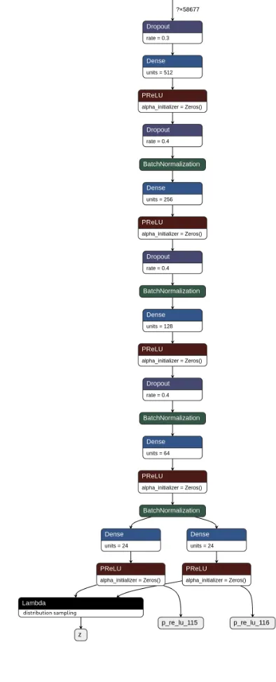
be the same as the input, thanks to the en- and decoding, it is possible to train both the encoder and decoder at the same time. The combination of the encoder and classifier results in the encoder-classifier. A graph representation of the encoder and the decoder can be seen in figure 1a and figure 1b

This setup allows for a pretrainedencoderby first training the autoencoder and then cutting of thedecoder part. This pretrainedencoder can then be used to create the encoder-classifier potentially improving performance and training time.

It is also possible to use a non-neural network classifier in combination with theencoder. The encoder is then used as a dimensionality reduction preprocessor. The encoder compresses the data into a lower dimension. This compressed data is then as input for the classifier. The combination of these models can however not be trained together to further optimize them like theencoder-classifier can.

1) Modified VAE loss: The reconstruction loss used to train the VAE will be heavily influenced by the large num-ber of missing values in this dataset. For example, during reconstruction, the network could generate a value of 1 for a certain variable that was missing. This means that the loss for this variable would be very high. However this is wrong because the network is doing what it is supposed to do, it is simply impossible to validate the generated variable. What we actually want is the network to learn only from the available data and not from the missing values.

We therefore propose a simple addition to the reconstruc-tion loss that takes missing values into considerareconstruc-tion, based on the work of Beaulieu-Jones et al. [15]. The pseudo-code can be seen in algorithm 1. The Modified VAE loss uses the normal VAE loss from equation 2 but for each input variable that is zero it will return a zero instead of calculating a reconstruction loss between that input variable and its related output variable. This approach makes sure that the network is only penalized for outcomes that are really wrong instead of missing.

ify6= 0 then

returnreconstructionErrorF unction(y,yˆ); else

return0; end

Algorithm 1:Modified VAE loss. Input is the original data (y) and and the recosntruced data (ˆy), if y is zero no loss is calculated

(a) Encoder network. Input starts at the top (encoder input). This network has three outputs that can be seen at the bottom. The outputs are, from left to right, p re lu 115 the latent mean , p re lu 115 the latent standard deviation and z the sampled vector from this mean and standard devaition.

(b) Decoder network. Input starts at the top z sampling. This network has one output that can be seen at the bottom. The output is a reconstructed representation based on input z sampling .

Fig. 1: Graph representations of the decoder and encoder networks. The autoencoder is created by connecting z from the encoder network to z sampling form the decoder network. Images were generated by Netron [31].

C. SGAN

The SGAN architecture can be divided into two main parts. The generator and the discriminator. The generator generates data from a randomly sampled vector of length 100. The discriminator classifies data on their class labels

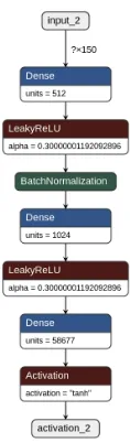
(a) Encoder network. Input starts at the top (input 2). This network has one output (activation 2) that can be seen at the bottom. The output is in the form of a generated customer.

(b) Decoder network. Input starts at the (top input 1). This network has one softmax output with the following labels [buy,not-buy,fake].

Fig. 2: Graph representations of the discriminator and generator that are important parts of the Sgan architecture. Images were generated by Netron [31].

activation for label classification or [fake] with a sigmoidal activation for fake data detection.

The SGAN is a bit different from a normal Neural Net-work in the way the training set up. every batch flows through the architecture two times. The pseudo-code from Odena [9], that can be seen in figure 3 illustrates this perfectly. Every batch first is doubled by adding generated data from the generator, creating a new batch with both generated and real data where generated and real are both equally represented. The D/C is then trained using this batch, note that the

generator weights are locked during this. After training of the D/C, the generator gets updated by feeding the generator a noise batch. The weights of the generator are then updated based on the output of the D/C, note that the D/C weights are locked during this.

D. Network training

Fig. 3: Copy of SGAN training algorithm from Odena [9]. In this copy D is the discriminator, D/C the combined discriminator, G the generator and classifier and NLL the negative log likelihood. See the paper of Odena [9] and the section II.

selecting the model from the epoch with the lowest validation loss. The training data was shuffled before every epoch. The batch size of every model was 32. The latent dimension size of the VAE unless stated otherwise was 24.

IV. EARLY RESULTS

A VAE was implemented based on the techniques provided by Kingma et al. [8] in order to explore the usability of a VAE on this dataset. During the unsupervised training a part of the data set was used that only included the numerical datatype. This part included the data of 4000 customers. This part was the only available data at the start of the research and is different from the set used during the final evaluation. The latent variables were constrained to three dimensions in order to visualize them. The visualization contains the encodings for every data point in a three-dimensional graph where every dimension corresponds to a latent variable. The data points were divided into three groups based on the age of the person due to the buying targets not being available yet. The graph can be seen in figure 4

By visually inspecting the graph it is clear that some clustering occurs. Even though the goal of this research is not to predict age groups and the fact that latent space was con-strained to 3 dimensions the VAE shows to be a promising method for doing dimensionality reduction on this dataset. It was therefore decided to continue with fully implementing and evaluating VAE’s using different parameters.

V. EVALUATION

The subset used for evaluation was created from the dataset provided by CB, more information about this dataset can be found in section I-A. More information about the data preparations can be found in section III-A. This data set contained 34289 customers with target labels equally repre-sented by under-sampling the minority class. Each customer had 4820 variables recorded. Of these variables an average of 97 percent are missing. The train and test set was were

Fig. 4: Latent vector visualisation of 4000 customers. Colors indicate customer age group.

created by splitting the dataset into 60 percent training set and 40 percent test set.

A. Dimensionality reduction

The dimensionality reduction capabilities of the VAE will be evaluated by multiple metrics. First the reconstruction loss, specifically the mean squared error of the input and output. A lower loss will show the ability of the network to reduce dimensions while keeping information loss at a minimum. And because a dimensionality reduction with the lowest information loss is preferred the network with the lowest reconstruction loss will be considered best.

Secondly the F1 [33] performance of classification when using the network as a preprocessor or pre-trained network. This F1 score can then be compared to a classifier that was trained on the original data. This will show the influence of information loss due to compression. The lowest influence or in other words the classifier with an F1 score that is closest to the F1 score of the classifier trained on the original data will be considered best. Note that only one target set is available, thus giving only an indication of this influence.

Lastly, the dimensionality reduction will also lead to de-creased file sizes and dede-creased classifier training time when the dimensionality reduction is used as a pre-processing step. The decreases in file size and training time are only beneficial if the previous metrics are satisfactory. The benefits have to be considered together in order to make a useful conclusion.

B. Influence of missing data on reconstruction

C. Neural network classification

The SGAN and the encoder-classifier networks can be used for classification directly. These networks are evaluated based on the F1 score.

VI. RESULTS

A. Parameters

In this section VAE configurations will be defined using three parameters. The first parameter is Loss function this parameter defines the loss function used, it can be either normalormodified see section III-B.1 for more information on this. The second parameter is Annealing this variable defines if annealing was used during training of the VAE, see section III-B.2 for more information. The last parameter is betawhich defines what beta was used during training, again see section III-B.2 for more information. When annealing was enabled the beta parameter defines the maximum value. In this document, these configurations have the same color in every graph.

A fourth parameter can be found in configurations that are used for classification either with a pre trained or preprocessor setup. This parameter is Classifier and defines the type of classifier used, the possible paramters areprecls, boostandrandomf.preclsdefines a neural network classifier using a pretrained encoder. boost refers to a Boosted Tree while randomf refers to a Random Forest using a VAE preprocessor.

B. VAE training

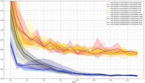
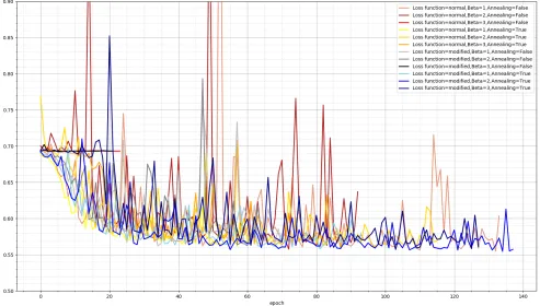
Figure 5 shows the training loss of every VAE configu-ration. Note that not all of the VAE losses can be directly compared because of the fact that some parameters altered the loss functions. Because of early stopping, not every configuration ends on the same epoch. the maximum number of epochs was set at 400. The lines indicate validation loss while the dotted lines indicate the training loss.

All of the configurations show a fast decrease of the loss within the first 20 epochs and a further stabilization up to epoch 50 after which no big decreases in loss can be observed. However, some configurations show a sudden drop in loss around the 100 epoch mark. The models seem to get stuck in a local minimum and then break out to get into a second local minimum.

Furthermore, before this sudden drop every configuration goes through at least one spike of very high loss, the validation loss quickly increases and decreases within a few epochs. However, overall the validation loss follows the training loss closely indicating no overfitting, the training loss is cannot be seen in the graph in order to keep the graph readable.

There is also a clear difference in loss between the con-figurations with the modified and the normal VAE loss. The configurations with the normal VAE loss have a generally higher training and validation loss. This difference could be explained by the exclusion of the missing variables in when using the modified loss, again it is hard to compare these loss functions directly due to the influence of the parameters

on the loss during training. Note that the loss is stable but far from zero, this could be due to the high number of missing values or that more optima remain.

Because the results from figure 5 only show the results of single training runs the training was repeated in order to get more reliable results. However, due to time constraints, these runs were limited to 20 epochs. Figure 6 shows the mean and standard deviation validation loss of every VAE configuration during training. The VAE’s were trained three times for 20 epochs each time. The standard deviation is depicted by the shaded area around the lines.

The results show to be the same as during the first 20 epochs of figure 5, the lines seem to stabilize at the same amount of epochs and there is a clear difference of eventual loss between the normal and modified VAE losses. The standard deviation during training is very low, meaning a low influence of chance. The parameters next to the two different VAE loss functions do seem to have an influence on the first few epochs but do not seem to have an influence later on because every configuration converges to the almost same loss value eventually. However, as noted earlier, it is not really possible to compare these eventual loss values because the parameters directly influence the outcome of the loss function.

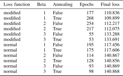
Loss function Beta Annealing Epochs Final loss modified 1 False 177 110.836 modified 1 True 268 109.899 modified 2 False 254 112.217 modified 2 True 217 112.075 modified 3 False 55 133.288 modified 3 True 53 133.691 normal 1 False 195 117.456 normal 1 True 175 117.606 normal 2 False 114 140.867 normal 2 True 128 140.856 normal 3 False 93 140.869 normal 3 True 98 140.868

TABLE I: VAE epoch amount and final training loss

Another view of the data from figure 5 can be seen in table I. This table shows the final validation loss of every configuration and the number of epochs the training ran. Because of early stopping, not every VAE trained for the same amount of epochs. It can be seen that the number of epochs varies heavily. VAE’s with annealing enabled are close to their constant beta counterparts for both the max epochs and the loss. This indicates that the Annealing has no influence on the loss during training after the beta reaches the maximum value. High beta values lead to higher final training loss in this table. Higher beta values also trained for fewer epochs.

C. Data reconstruction

Fig. 5: VAE validation loss during the training of different VAE configurations. The red and orange lines are the configurations with the modified loss function while the bluer and grey lines are the configurations with the normal loss function. The Beta values are indicated by the hardness of the color.

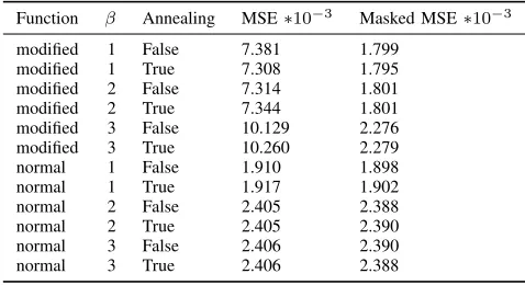
Function β Annealing MSE∗10−3 Masked MSE∗10−3

modified 1 False 7.381 1.799 modified 1 True 7.308 1.795 modified 2 False 7.314 1.801 modified 2 True 7.344 1.801 modified 3 False 10.129 2.276 modified 3 True 10.260 2.279 normal 1 False 1.910 1.898 normal 1 True 1.917 1.902 normal 2 False 2.405 2.388 normal 2 True 2.405 2.390 normal 3 False 2.406 2.390 normal 3 True 2.406 2.388

TABLE II: MSE and Masked MSE reconstruction error of each VAE configuration. Each VAE configuration had a single training run with a maximum of 400 epochs.

accurately. The masked MSE works like the Modified loss function by ignoring missing values, see III-B.1 for more information. The VAE’s used for this were the same as the VAE’s in the previous training results.

The reconstruction loss of different VAE’s after training for a maximum of 400 epochs can be seen in table II. In table II it can be seen that the losses of the annealing

configuration are very close to its non-annealing counterpart, this is consistent with the results form table I and indicates that the Annealing has no influence on the loss during training after the beta reaches the maximum value.

Furthermore the masked losses are consistently lower than the normal losses when the modified VAE loss function is used during training. This was to be expected because the configurations with the modified loss are trained and therefore optimized using this error. It should therefore also perform better when using this error.

There is no clear difference between masked a normal loss when a normal VAE loss function is used. This means that on average the usage of the modified loss does not impact the performance on all of the variables while performing better on the non-missing variables.

Fig. 6: VAE mean validation loss and mean training loss during the training of different configurations and limited to 20 epochs. The red and orange lines are the configurations with the modified loss function while the bluer and grey lines are the configurations with the normal loss function. The Beta values are indicated by the hardness of the color.

Function β Annealing MSE∗10−3 Masked MSE∗10−3

modified 1 False 11.596±0.005 2.308±0.005 modified 1 True 11.629±0.025 2.306±0.004 modified 2 False 11.648±0.107 2.309±0.003 modified 2 True 11.595±0.100 2.306±0.006 modified 3 False 11.592±0.118 2.308±0.006 modified 3 True 11.623±0.015 2.308±0.003 normal 1 False 2.491±0.005 2.441±0.019 normal 1 True 2.480±0.008 2.449±0.004 normal 2 False 2.491±0.004 2.449±0.011 normal 2 True 2.490±0.004 2.447±0.005 normal 3 False 2.495±0.005 2.455±0.014 normal 3 True 2.486±0.008 2.454±0.007

TABLE III: Mean and standard deviation of the MSE and Masked MSE reconstruction error of each VAE configura-tion. Each VAE configuration had three training runs with each training run having a maximum of 20 epochs.

The reconstruction loss of different VAE’s after training for 20 epochs can be seen in table III. The results show the mean and standard deviation of the MSE and Masked MSE reconstruction error of each VAE configuration. Each VAE configuration had three training runs with each training run having a maximum of 20 epochs

When training for only 20 epochs no clear distinctions can be seen. The only clear divide is between the two types of VAE losses. The modified VAE loss performs slightly better using the masked MSE while the normal VAE loss performs better using the normal MSE, again this is expected. The overall standard deviations are very low. Comparing this table with table II shows that the MSE and masked MSE decrease even further after training for more epochs. The configurations with the modified loss however have a relatively bigger decrease when comparing the results from epoch 20 and the final epoch

These results show that the difference between the modi-fied loss and the normal loss already have an impact on the resulting error as early as 20 epochs. Also, the configurations with the modified loss benefit more from more epochs when looking to the reconstruction losses. The low standard deviations show that these results are repeatable.

D. Changes to error function

Loss function Beta Annealing Error Masked Error modified 1 False 0.250 0.037 modified 2 False 0.249 0.038 modified 3 False 0.297 0.034 normal 1 False 0.050 0.215 normal 2 False 0.059 0.234 normal 3 False 0.059 0.236

TABLE IV: Normal and masked reconstruction error, as covered in section VI-D, of each VAE configuration.

cross-entropy (BCE) and root mean squared error (RMSE) was chosen. The formula can be seen in 4.

Error= 1 n

n

X

i=1

BCE(ybi,yˆbi) +RM SE(yci,yˆci) (4)

Whereybi andyci are the binary and continuous datapoints

respectively.

The VAE configurations from the previous chapter were then reevaluated using this new error function. While retrain-ing the configurations with this error function as the basis for the loss functions would be possible it was not done due to time constraints. The configurations with annealing were not evaluated in these results due to time constraints and the fact these configurations do not show clear differences compared to the non-annealing configurations after training in the previous sections.

The results of the evaluation of the reconstruction with the new error function can be seen in table IV. The VAE configurations with the modified loss function show to have a significantly lower error using the masked error compared to the configurations with the normal loss function. When looking at the normal error however the configurations with the modified loss function show to have a significantly higher error compared to the configurations with the normal loss function. This is different from the results from table II where the configurations with the modified loss always performed the same or better. Like in the tables from the previous sections a lower beta value generally leads to a lower error.

E. Influence of missing data

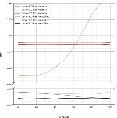
In this section, the influence of missing data on the model is explored by creating artificial missing data. The artificial missing data is created by replacing non-missing data with a 0. By comparing the reconstructed output with the original, before replacing that is, it can be observed how the model reacts to more missing data. One possibility would be that the model starts to impute the missing values because it learned the relations between variables and can therefore predict what variable could be in place of the missing. Another possibility is that the model simply starts performing worse. The error used in this section is the error described in section VI-D.

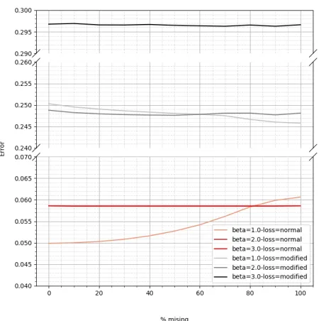
Figure 7 shows the error of the reconstructed represen-tation compared to the original when using different VAE configurations and different percentages of variables replaced by zeros. In this graph, all of the VAE configurations seem to

Fig. 7: Reconstruction error after replacing variables with zeros. The error function used can be found in section VI-D. Note that this figure has broken axes.

perform better when the amount of missing data is increased except for the configuration with a beta of 1 and using the normal loss function where the error increases somewhat. The configurations with the normal loss function and with a beta value of two and three stay completely flat, this is possibly due to the network learning more of the distribution of the variables instead of the relations between variables. The configurations with a lower beta and the modified loss function react somewhat to the added missing values by a small decrease of error. Furthermore keep in mind that 93% of variables are missing, heavily clouding these results.

Figure 8 is the same as the previous figure, however, before calculating the loss the data is filtered by only selecting the values that are non-missing in the original removing the big influence of all of the missing data. Again his mask somewhat resembles the modified loss of section III-B.1. Due to this resemblance, the configurations with the modified loss function have a significantly lower error compared to the configurations with the normal loss function. The error of the configurations with the modified loss is also significantly lower when comparing it with the previous figure, figure 7, while the configurations with the normal loss function have significantly higher error compared to figure 7. This can also be observed in table IV

Fig. 8: Reconstruction error after replacing variables with zeros, filtered by only selecting the values that are non-missing in the original.The error function used can be found in section VI-D. Note that this figure has broken axes.

the added missing values by a small decrease of error. Figure 9 is the same as the previous figures, however, the data is filtered by only selecting the values that were replaced by missing. The error of the VAE configurations with the normal loss function is generally higher in this graph. All of the models react to the increase of added missing values by an increase of loss. The configurations with the higher beta values find some kind of optimum pretty fast while the configurations with the lower beta values continue to rise up until there are only missing values.

Looking at all three figures in this section, the models do not seem to learn much about the relations between variables in this dataset. The straight lines indicate that the model learns more about the distribution of each variable. When looking at the configurations with the modified loss function it is clear that the masked reconstruction error is consistently lower. The modified loss function is therefore successful in forcing the model to learn more about the non-missing data points.

F. Classification baseline

The original data was used to train a Random forest [11] and a Boosted Tree [12]. The F1 performance of these models was used as a baseline for the models trained and evaluated on the encoded representations.

The baseline F1 score can be seen in table V. Both models perform close to each other. The mean classification F1 score of the SGAN after training for 200 epochs was 0.72 as can be seen in table V. This is very close to the performance of the boosted tree and random forest. The fact that a state

Fig. 9: Reconstruction error after replacing variables with zeros, filtered by only selecting the values that were replaced by missings.The error function used can be found in section VI-D.

Random Forest Boosted Tree SGAN F1 .72 .73 .72

TABLE V: Average F1 performance of classifiers on original data (not encoded or compressed)

of the art neural network cannot improve the classification performance over the decision tree-based models indicates that the data might not have complex relations or structures in it.

G. Classification using VAE preprocessor

This section describes the performance of different classi-fiers when trained and evaluated not on the original dataset but on the encoded representation created by one of the VAE configurations. This was done by only using the encoder of a fully trained VAE and using it as a preprocessor that can encode data with minimal information loss. More technical information can be found in section III-B. The best case scenario would be a classifier that performs just as good as the baselines from VI-F while using the encoded data representations.

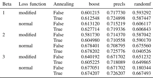
Beta Loss function Annealing boost precls randomf 1 modified False 0.601215 0.717730 0.593292 True 0.612548 0.724898 0.587447 normal False 0.613120 0.715219 0.606117 True 0.627714 0.719336 0.606843 2 modified False 0.581730 0.714370 0.587042 True 0.604980 0.710558 0.590170 normal False 0.678401 0.708795 0.675560 True 0.678202 0.725776 0.040526 3 modified False 0.640192 0.671702 0.651232 True 0.605225 0.718089 0.649865 normal False 0.677051 0.671702 0.180344 True 0.674207 0.726207 0.667493

TABLE VI: F1 performance of classifiers trained and eval-uated on encoded representations (boost and randomf). F1 performance of classifiers trained and evaluated on encoded representations (precls) The VAE’s trained for usage as pre-processors were limited using early stopping to 400 epochs

Beta Loss function Annealing boost randomf 1 modified False 0.647±0.011 0.660±0.006

True 0.649±0.013 0.666±0.005 normal False 0.654±0.006 0.664±0.010 True 0.632±0.018 0.642±0.021 2 modified False 0.666±0.011 0.672±0.020 True 0.640±0.009 0.662±0.009 normal False 0.597±0.074 0.647±0.018 True 0.589±0.069 0.654±0.011 3 modified False 0.611±0.054 0.647±0.009 True 0.616±0.047 0.650±0.010 normal False 0.616±0.029 0.659±0.005 True 0.638±0.028 0.651±0.016

TABLE VII: Mean F1 performance of classifiers trained and evaluated on encoded representations. The VAE’s trained for usage as preprocessors were limited using early stopping to 20 epochs

tree classifiers is negligible. Contrary to the previous sections a higher beta value leads to higher performance overall.

The classification performance of the classifiers on differ-ent VAE preprocessors after training for 20 epochs can be seen in table VII. The results show the mean and standard deviation of 3 training runs. Even after 20 epochs, the encoded representations perform very close to the baseline. In this table the modified VAE loss based models perform a bit better overall. Overall the standard deviation is quite low, with some exceptions, meaning high reliability. Differ-ence between the random forest classifiers and boosted tree classifiers is negligible. In these results, the beta parameter does not have much influence.

All dimensions Encoded representation RandomForest 41 sec 2.4 sec

BoostedTree 37 min 7 sec

TABLE VIII: Training time of classifiers

The training time of different classifiers is also decreased when using encodings as can be seen in table VIII. The Random forest is faster overall, but that has to do with the

parallel training compared to the sequential nature of the boosted tree. The difference between original and Encoded is quite big however, the classifiers train more quickly on the encoded representation. This was of course expected due to the simple fact that fewer variables mean faster training. However, this does not undermine the practical benefit that the encoding of data has on the speed of classification and training.

The difference in performance between classifiers trained and evaluated on the original en the encoded data is rela-tively small. This means that next to encoding information needed for reconstruction, the goal of the VAE, the VAE is also encoding useful for classification. Classification and representation, therefore, have some information shared but are not exactly the same as can be observed by the influence of the beta parameter in these results. No clear difference between classifier types can be seen in these results.

H. Preprocessor data compression

When the encoder of a VAE is used as a preprocessor it could be seen as a data compression algorithm tailored to the dataset is wat trained on. In this section, the generic compression technique Zip is compared to the preprocessor.

Size original size zipped Original 376MB 2.5MB Encoded 396KB 365KB

TABLE IX: Compressed and uncompressed file size of 4000 customers

When file sizes of the data from 4000 customers are compared between original and encoded representation it is clear that the encoded representation uses significantly less memory. This can be seen in table IX. When the original and its encoded representation are compressed using Zip the difference is significantly less big. While the zipped data uses less memory than the original data, the zipped data needs to be unzipped prior to using it. Therefore negating the benefits of zip compression for practical usage. The original data and the encoded representations were saved to the HDF5 [34] file format without any compression.

The fact that the zip algorithm is unable to compress the encoded representation any further indicates that the encoder is able to compress the data into multiple unique features, thus retaining as much information as possible. This experiment however does no show the quality of these features.

I. Classification using pretrained VAE

Fig. 10: Validation loss during training of different configurations of a pre trained neural network.

of weights that are already optimized for the dataset and a similar goal. These weights can then be improved further in the classification network by doing more training.

Figure 10 shows the validation loss during the training of different pre-trained classifiers. It is clear that every configuration eventually reaches the same optimum with two exceptions that seem to get stuck almost immediately. While not in the graph the validation loss is generally lower than the training loss.

Figure 11 shows the F1 validation during the training of the same classifiers as figure 10. The F1 performance also reaches an optimum quickly with again two exceptions which seem to get stuck immediately. The validation performance is generally higher than the training performance.

Figure 12 shows a zoomed-in version of figure 11 with only 3 configurations present in order to show the influence of a beta of three. The configuration with the higher beta takes more epochs to get to the same performance as the other two configurations. This could explain the two flat lines in figure 11 that also have a beta of 3.

Interestingly these 2 lines both had annealing disabled when training the VAE. This indicates that the annealing does have an effect on the eventual VAE even after the beta value has its maximum value. While Annealing did not have any noticeable effect on the reconstruction and classification

using a preprocessor performances, it does have an effect on the model’s ability to update its weights towards a new task. Table VI shows the F1 test performance of the classifiers after training on the test set. These results correspond to the results of the previous two figures. Most classifiers performed the same with the exception of the two classifiers that did not seem to train. These classifiers both had annealing disabled and a beta of 3. They have significantly lower F1 scores. On average the F1 performance is comparable to the results of table V. Overall the F1 performance is slightly higher when using the modified loss function during pre-training.

It is clearly possible to use an encoder from a VAE as a pretrained part of a classification network. The parameters used during the training of the VAE do seem to have less of an influence on the classification performance, contrary to the results of the preprocessor setups. The beta has an influence on the speed of which the network is able to get to an optimum or to even get to an optimum at all. A high beta makes the network untrainable, however, the enabling of annealing makes it trainable again. The loss function does to not have any influence.

VII. DISCUSSION

Fig. 11: Validation F1 performance during training of different configurations of a pre trained neural network.

training a VAE for 400 epochs compared to its counterpart with a constant beta. The KL-annealing also has no measur-able impact on the classification performance when training for a VAE 400 epochs compared to its counterpart with a constant beta. This is to be expected because the annealing is only done for the first 10 epochs. In other words after 10 epochs a VAE with a beta of 3 has the same loss function as a VAE with annealing enabled and a maximum beta of 3. This becomes clearer when looking at the results of the VAE’s that were trained for 20 epochs. Furthermore based on the current results the KL-annealing does not influence the number of epochs needed for an optimal loss.

The only big influence of KL-annealing was during fine-tuning of the pre-trained networks. Configurations with a beta of 3 and with annealing disabled did not learn at all and therefore also have a significantly lower performance score compared to their annealing counterparts or configurations with lower beta values. However these higher beta values do not result in better classification performance, the influence of KL-annealing is therefore of no benefit.

The loss function used when training the VAE does not show to have a significant influence when looking at the pre-trained and preprocessor classification setups. It does, however, have a huge influence on the reconstruction errors. As expected, the modified loss performs better when

evalu-ating with the masked errors while the normal loss function performs better when evaluating with the normal errors. The modified loss, therefore, forces the network to focus on the data that is available. But this has no measurable influence on the classification tasks, at least in this dataset.

The loss function and annealing used during training of the VAE are not used during fine-tuning. It therefore has no direct influence during fine-tuning. The only influence of these parameters would be a VAE that has overcome some local optimums which would lead to better performance after fine-tuning. This could be one of the reason for the inability to learn during finetuning as covered previously.

A high beta decreases the number of epochs during VAE training due to the fact that early stopping stops the training. A higher Beta increases the number of epochs needed for getting to an optimum during fine-tuning of a pre-trained network or even impeding the ability to learn something at all. The optimum of every parameter configuration is eventually the same, except for the models that did not learn anything. It can be therefore concluded that purely for classification purposes and a decreased training time a lower beta is preferred. When looking at reconstruction a low beta also performs better. However when looking at classification using a pre-processor, a higher beta is preferred.

Fig. 12: Validation F1 performance during training of different configurations of a pre trained neural network during the first 30 epochs.

forces the network learn not only reconstruction but re-construction with latent variables that conform to a certain distribution. This is of course not useful when solely evaluat-ing reconstruction. The reason for the pre-trained networks benefitting form a high beta and the preprocessing classi-fiers benefitting form a low beta is that the preprocessing classifiers are stuck with an encoder that is optimized for reconstruction, which is not optimal. An encoder trained with a high beta is however less optimized for reconstruction which leads to better classification. The pre-trained networks can overcome this by re-optimizing during fine-tuning.

When introducing more missing values by artificially creating more the reconstruction error did not change much when looking at all of the variables. This is consistent with the results of Ennett et al. [5] where it was not possible to find a breaking point of the models. This is due to the ability of autoencoders to generate reconstructions that are, in simple terms, averages of the data distribution when no or few input neurons are activated. This means that the VAE configurations capture distribution more than structure even when using the modified loss function.

Because of only a single observation is available of the different VAE configurations trained for 400 epochs chance could have a big impact on the conclusions. The fact that the

annealing and non-annealing counterparts perform similarly removes this chance problem somewhat. Next to that early stopping was also used which ended the training of some configurations as early of 50 epochs. It might be possible that these configurations were not done training but simply dealing with local optimums or slow learning overall.

VIII. CONCLUSION

According to the results a VAE can be implemented as a dimensionality reduction prepossessing step for classifica-tion. Successful classification can still be done with only minimal loss in performance. Classifiers using the VAE as a pre-processor perform almost as well as classifiers trained on all of the variables. The type of classifier is not important. Networks with pretrained encoders from the VAE were on par with the classifiers trained on all of the variables. The VAE is therefore able to reduce dimensionality while keeping the most of the important information needed to make a reconstruction or a classification.

compression every algorithm could then be updated or re-trained. Leading to a decrease in total computational power and total memory needed.

For classification using a pre-trained encoder a low beta value is preferred while classification using an encoder as preprocessor benefits from a high beta value. The type of loss function has no influence on the classification performance, however, for reconstruction purposes, the modified loss func-tion is able to get better performance on non-missing data. That said, overal both types of models show to learn more about the distribution of the data than its structure The usage of KL-annealing does not have any benefit for classification. The classification performance of the SGAN was not an improvement over the performance of the boosted tree or the random forest. It is possible that the data simply does not contain highly complex relations that can normally only be modeled by a deep neural network.

IX. FUTURE WORK

An interesting topic for future work would be exploring the benefits of having the generator of the SGAN also generate data labels. This was also proposed in the paper of Odena. In this setup the discriminator could do a 2 sided classification where it would classify Fake/Real and the class label at the same time.

As an added benefit data will be anonymous after dimen-sionality reduction. This could be explored more in future work. For example, by giving data scientist with lower security levels access to confidential data by giving them the encoded version only. These scientists could then exper-iment with different algorithms and techniques. It would be interesting to research if algorithms trained on the encoded data could be transferred or adapted to the original data, in order to get optimal performance after the experimentation phase.

An interesting approach to explaining the classification models that will be trained in this research by using the lo-cal interpretable model-agnostic explanations (LIME) model provided by Ribeiro et al. [35]. The biggest advantage of LIME is it is not model dependent. Furthermore, LIME results are easily interpreted by humans.

Future work should verify these conclusions by rerunning the experiment multiple times with shuffled sets for training, validation and testing between each run. Future work should also validate the classification abilities of the VAE by eval-uating the systems of this paper on different classification tasks than the single task evaluated in this paper. Lastly, the VAE configurations should be trained with a fixed epoch length.

The decoder part of the VAE’s was not separately eval-uated in this research for reasons explained in the related work. However, a decoder could be used in multiple ways, for example, data generation. Furthermore, the decoder has an impact on the reconstruction loss, researching the decoder separately could give insights on why the VAE performs in a certain way when reconstructing data or how to improve the learning of the VAE.

Continuing with improving the learning of the VAE, it would also be useful to explore the performance of the VAE loss function when the MSE is replaced with the error function described in section VI-D.

This research focused on the VAE. However, in some cases, a lower beta value was beneficial compared to a higher beta. It would be therefore also worthwhile to look into using a beta value of zero. Effectively a VAE into an autoencoder. As an alternative to the VAE, an Adversarial Autoencoder (AEE) [36] could be implemented and evaluated. The AEE uses techniques first proposed by the GAN framework to train an autoencoder in an adversarial manner. Like the VAE this network can also be used for dimensionality reduction and semi-supervised learning.

REFERENCES

[1] David Silver et al. “Mastering the game of Go with deep neural networks and tree search”. In: nature 529.7587 (2016), p. 484.

[2] Pedro J Garc´ıa-Laencina, Jos´e-Luis Sancho-G´omez, and An´ıbal R Figueiras-Vidal. “Pattern classification with missing data: a review”. In: Neural Computing and Applications19.2 (2010), pp. 263–282.

[3] John W Graham. “Missing data analysis: Making it work in the real world”. In: Annual review of psychology60 (2009), pp. 549–576.

[4] Gerard V Trunk. “A problem of dimensionality: A simple example”. In: IEEE Transactions on Pattern Analysis & Machine Intelligence 3 (1979), pp. 306– 307.

[5] Colleen M Ennett, Monique Frize, and C Robin Walker. “Influence of missing values on artificial neu-ral network performance”. In:Medinfo. 2001, pp. 449– 453.

[6] Herv´e Abdi and Lynne J. Williams. “Principal com-ponent analysis”. In:Wiley Interdisciplinary Reviews: Computational Statistics 2.4 (June 2010), pp. 433– 459. DOI: 10 . 1002 / wics . 101. URL: https : //doi.org/10.1002/wics.101.

[7] Charles X Ling and Victor S Sheng. “Cost-Sensitive Learning and the Class Imbalance Problem”. In: (). [8] Diederik P Kingma and Max Welling.Auto-Encoding

Variational Bayes. 2013. arXiv:1312.6114. [9] Augustus Odena. “Semi-supervised learning with

generative adversarial networks”. In: arXiv preprint arXiv:1606.01583(2016).

[10] Tim Salimans et al. “Improved techniques for training gans”. In:Advances in Neural Information Processing Systems. 2016, pp. 2234–2242.

[11] Tin Kam Ho. “The random subspace method for constructing decision forests”. In:IEEE Transactions on Pattern Analysis and Machine Intelligence 20.8 (1998), pp. 832–844.DOI: 10.1109/34.709601.

[12] Jerome H Friedman. “Stochastic gradient boosting”. In: Computational statistics & data analysis 38.4 (2002), pp. 367–378.

[13] Dumitru Erhan et al. “Why does unsupervised pre-training help deep learning?” In:Journal of Machine Learning Research11.Feb (2010), pp. 625–660. [14] Cheng-Yuan Liou, Jau-Chi Huang, and Wen-Chie

Yang. “Modeling word perception using the Elman network”. In:Neurocomputing 71.16-18 (Oct. 2008), pp. 3150–3157.DOI:10.1016/j.neucom.2008. 04.030. URL: https://doi.org/10.1016/ j.neucom.2008.04.030.

[15] Brett K Beaulieu-Jones and Jason H Moore. “Miss-ing data imputation in the electronic health record using deeply learned autoencoders”. In: Pacific Sym-posium on Biocomputing 2017. World Scientific. 2017, pp. 207–218.

[16] S. Kullback and R. A. Leibler. “On Information and Sufficiency”. In: The Annals of Mathematical Statis-tics 22.1 (Mar. 1951), pp. 79–86. DOI: 10 . 1214 / aoms/1177729694. URL: https://doi.org/ 10.1214/aoms/1177729694.

[17] Irina Higgins et al. “beta-vae: Learning basic visual concepts with a constrained variational framework”. In:International Conference on Learning Representa-tions. 2017.

[18] Samuel R. Bowman et al. “Generating Sentences from a Continuous Space”. In: (2015). arXiv:1511. 06349.

[19] Harri Valpola.From neural PCA to deep unsupervised learning. 2014. arXiv:1411.7783.

[20] Antti Rasmus et al. Semi-Supervised Learning with Ladder Networks. 2015. arXiv:1507.02672. [21] Mohammad Pezeshki et al. “Deconstructing the ladder

network architecture”. In:International Conference on Machine Learning. 2016, pp. 2368–2376.

[22] Ian J. Goodfellow et al.Generative Adversarial Net-works. 2014. arXiv:1406.2661.

[23] Lucas Theis, A¨aron van den Oord, and Matthias Bethge. “A note on the evaluation of generative mod-els”. In:arXiv preprint arXiv:1511.01844(2015). [24] Kai Ming Ting. “Inducing cost-sensitive trees via

instance weighting”. In: European Symposium on Principles of Data Mining and Knowledge Discovery. Springer. 1998, pp. 139–147.

[25] Haibo He et al. “ADASYN: Adaptive synthetic sam-pling approach for imbalanced learning”. In: Neural Networks, 2008. IJCNN 2008.(IEEE World Congress on Computational Intelligence). IEEE International Joint Conference on. IEEE. 2008, pp. 1322–1328. [26] Nitesh V Chawla et al. “SMOTE: synthetic minority

over-sampling technique”. In: Journal of artificial intelligence research16 (2002), pp. 321–357. [27] Eric Jones, Travis Oliphant, Pearu Peterson, et al.

SciPy: Open source scientific tools for Python. [On-line; accessed ¡today¿]. 2001–. URL: http://www. scipy.org/.

[28] Franc¸ois Chollet et al.Keras.https://keras.io. 2015.

[29] Raoul Fasel. Repository for code used in adapting the variational auto encoder for datasets with large amounts of missing values.[Online; accessed ¡today¿]. 2019. URL: https : / / gitlab . com / vae _ missing_values.

[30] J. Sola and J. Sevilla. “Importance of input data normalization for the application of neural networks to complex industrial problems”. In:IEEE Transactions on Nuclear Science44.3 (June 1997), pp. 1464–1468.

DOI: 10 . 1109 / 23 . 589532. URL: https : / / doi.org/10.1109/23.589532.

[31] Lutz Roeder et al. Netron - Visualizer for deep learning and machine learning models. https : / / github.com/lutzroeder/netron. 2019. [32] Timothy Dozat. “Incorporating nesterov momentum

into adam”. In: (2016).

[33] Yutaka Sasaki et al. “The truth of the F-measure”. In: Teach Tutor mater1.5 (2007), pp. 1–5.

[34] The HDF Group.Hierarchical Data Format, version 5. http://www.hdfgroup.org/HDF5/. 1997-NNNN. [35] Marco Tulio Ribeiro, Sameer Singh, and Carlos

Guestrin. “”Why Should I Trust You?”: Explaining the Predictions of Any Classifier”. In:Proceedings of the 22nd ACM SIGKDD International Conference on Knowledge Discovery and Data Mining, San Fran-cisco, CA, USA, August 13-17, 2016. 2016, pp. 1135– 1144.