warwick.ac.uk/lib-publications
A Thesis Submitted for the Degree of PhD at the University of Warwick
Permanent WRAP URL:
http://wrap.warwick.ac.uk/94732
Copyright and reuse:
This thesis is made available online and is protected by original copyright. Please scroll down to view the document itself.
Please refer to the repository record for this item for information to help you to cite it. Our policy information is available from the repository home page.
Three Essays on Intertemporal Choice
by
Lisheng He
Thesis
Submitted in partial fulfilment of the requirements for the
Doctor of Philosophy
CONTENTS
CONTENTS ... i
List of Tables ... v
List of Figures ... vi
Acknowledgements ... x
Declarations ... xi
Abstract ... xii
CHAPTER 1 INTRODUCTION ... 1
1.1 Normative Models ... 3
1.1.1 Converging interest rates... 3
1.1.2 Intertemporal allocation of consumption ... 6
1.1.3 Intertemporal choice... 7
1.1.4 Forms of discount functions ... 9
1.1.5 Optimal choice when borrowing and lending rates differ ... 12
1.1.6 Interim summary ... 14
1.2 Empirical Findings ... 14
1.2.1 Monetary outcomes ... 15
1.2.2 Non-monetary outcomes ... 18
1.3 Causes of Departures from the Normative Models ... 19
1.3.1 Market imperfection and complication ... 19
1.3.2 Background consumption... 20
1.3.3 Uncertainty associated with delayed offers... 21
1.3.4 Subjective perception of delays ... 21
1.3.5 Myopia or a lack of self-control ... 21
1.3.6 Cognitive inertia ... 22
1.4 Cognitive Processes in Intertemporal Choice ... 22
1.4.1 Evaluation rule ... 23
1.4.2 Attention ... 24
1.4.3 Background contrast... 24
1.5 Overview of the Following Chapters ... 25
CHAPTER 2 A COMPREHENSIVE MODEL COMPARISON ... 27
ii
2.2 Models ... 28
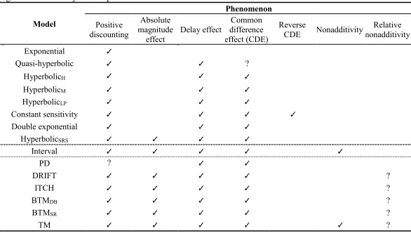
2.3 Behavioural Regularities and Model Coverage ... 33
2.3.1 Positive discounting ... 33
2.3.2 Absolute magnitude effect ... 33
2.3.3 Delay effect ... 34
2.3.4 Common difference effect and its reversal ... 34
2.3.5 Nonadditivity of intervals ... 34
2.3.6 Relative nonadditivity ... 35
2.3.7 Interim summary ... 35
2.4 Incomparability of Past Results ... 36
2.5 Methods ... 37
2.5.1 Data sets ... 37
2.5.2 Models ... 39
2.5.3 Stochastic specifications ... 39
2.5.4 Baseline model ... 40
2.5.5 Bayesian Information Criterion... 40
2.6 Results ... 41
2.6.1 Data screening ... 41
2.6.2 Stochastic specification influencing model performance ... 43
2.6.3 Model performance with the best-performing stochastic specification ... 44
2.6.4 Model performance with monolithic stochastic specifications ... 51
2.7 Discussion ... 53
2.7.1 Attribute-based models as the convincing winner ... 53
2.7.2 The importance of stochastic specifications in choice modelling ... 54
2.7.3 Conclusion ... 56
CHAPTER 3 ATTENTION AND INTERTEMPORAL CHOICE ... 57
3.1 Existing Literature ... 58
3.2 Framework of the Attention Effects ... 60
3.3 Attention Manipulation and the Present Study ... 62
3.4 Experiment 1: Varying LL Components ... 63
3.4.1 Experiment 1: Methods ... 63
3.4.2 Experiment 1: Results and discussion ... 67
3.5.1 Experiment 2: Methods ... 71
3.5.2 Experiment 2: Results and discussion ... 72
3.6 Discussion ... 76
CHAPTER 4 DETECTED PATTERNS OF IMPATIENCE ... 78
4.1 A Design Bias ... 79
4.2 An Order Effect ... 80
4.3 The Present Study ... 81
4.4 Experiment 1: Design Bias ... 84
4.4.1 Experiment 1: Methods ... 84
4.4.2 Experiment 1: Results and discussion ... 85
4.5 Experiment 2: Order Effect ... 91
4.5.1 Experiment 2: Methods ... 91
4.5.2 Experiment 2: Results and discussion ... 92
4.6 Discussion ... 95
4.6.1 Complexity and heterogeneity of the pattern of impatience ... 95
4.6.2 Methodological factors influencing the pattern of impatience ... 97
4.6.3 Conclusion, limitations and future directions ... 97
CHAPTER 5 GENERAL DISCUSSION ... 99
5.1 Summaries of the Findings ... 99
5.1.1 Evaluation rules ... 100
5.1.2 Attention effects ... 100
5.1.3 Background contrast effects ... 100
5.2 Theory Development Revisited ... 101
5.2.1 Static models ... 101
5.2.2 Dynamic models... 102
5.2.3 A theory gap ... 103
5.3 Extensions to Other Domains of Intertemporal Choice ... 103
5.3.1 Other response modes ... 104
5.3.2 Sequences ... 104
5.3.3 Losses ... 106
5.3.4 Non-monetary goods ... 106
5.4 Conclusion ... 107
REFERENCES ... 108
iv
Appendix 2A ... 130
Method for maximum likelihood search ... 130
Appendix 2B ... 131
Summary statistics of the 256 data sets involved in the model comparison .... 131
Appendix 2C ... 152
Parameter Space Partitioning Search ... 152
Appendix 2D ... 155
Relative nonadditivity ... 155
Appendix 3A ... 159
Cognitive Reflection Test ... 159
Appendix 3B ... 160
Demographic information questions ... 160
Appendix 3C ... 162
Results relating to cognitive reflection ... 162
Appendix 4A ... 165
Consideration of Future Consequences scale ... 165
Screening items for Experiment 1 in Chapter 4 ... 169
Appendix 4C ... 170
List of Tables
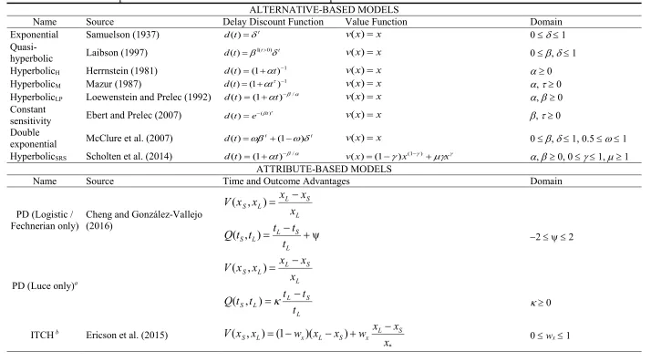
Table 2.1 Categories of intertemporal choice models. ... 28
Table 2.2 List of intertemporal choice models involved in this model comparison. . 30
Table 2.3 Behavioural regularities covered by intertemporal choice models. ... 32
Table 2.4 List of stochastic specifications. ... 39
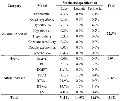
Table 2.5 Percentage of data sets identifying each combination of model and stochastic specification as producing the lowest BBIC value. ... 46
Table 3.1 Model evaluation and parameter estimation (Experiment 1) ... 69
Table 3.2 Model evaluation and parameter estimation (Experiment 2). ... 73
Table 4.1 Intertemporal choice items and implied hyperbolic discount rates in both the no-FED (front-end delay = 0) condition and the FED (front-end delay = 100) condition. ... 83
Table 4.2 Spearman correlation coefficients between the interval (t) and the absolute/proportional amount differences in the original Monetary Choice Questionnaire. ... 86
Table 4.3 Data from an example pair of items showing decreasing impatience. ... 87
Table 4.4 Parameter estimation for Experiment 2. ... 93
Table A1 List of the data sets involved in the model comparison in Chapter 2. ... 132
Table A2 Search dimensions and domains for the double-exponential discounting model. ... 152
Table A3 Search dimensions, domains and examples for the intertemporal choice heuristics model (ITCH)... 154
Table A4 Parameter estimation from models involving cognitive reflection. ... 162
vi
List of Figures
Figure 1.1. Indifference curves and marginal rates of intertemporal substitution (RA
and RB) of the two players at their initial endowments. Both players are
willing to trade with each other at certain rate (to reach a better
indifference curve) until their marginal rates of intertemporal substitution converge. ... 5 Figure 1.2. The optimal allocation of consumption to the two periods. ... 7 Figure 1.3. The budget constraint lines of two options with different net present
values. Option X is preferred to Option Y at their initial endowments, but the budget constraint line from Option Y (blue dashed) dominates the counterpart from Option X (orange dashed) according to the interest rate in the market. ... 8 Figure 1.4. Time-inconsistent allocations of consumption over time (Strotz, 1955). 10 Figure 1.5. Time-inconsistent choice between different goods when discount rates
differ across goods. ... 11 Figure 1.6. Optimal choice when borrowing and lending rates differ. The orange
dashed line is the budget constraint from receiving $1000 today (SS), with the saving interest rate of 1% per annum. The blue dashed line is the budget constraint from receiving $1100, with the borrowing interest rate of 20% per annum (LL). ... 13 Figure 1.7. A graphical illustration of Simonson and Tversky’s (1992) study on the
background contrast effect. ... 25 Figure 2.1. Details of the data sets. (a) Histogram showing implied daily interest
rates on a log-scale. (b) Scatterplot showing the distribution of the number of items (x-axis) and the average number of participants (y-axis) in the data sets, both on log-scales. ... 42 Figure 2.2. Differences in Aggregate BIC values between stochastic specifications.
(a) Differences between the Luce specification and the Logistic
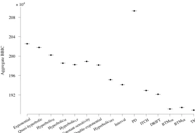
Figure 2.3. Aggregate BBIC value for each model q (ABBICq). ... 45
Figure 2.4. Pairwise differences in BBIC values (BBICqs) between the full tradeoff
model (TM) and other attribute-based models. The 225 data sets are ordered from the most negative difference (favouring another attribute-based model other than TM) to the most positive difference (favouring TM). Dashed lines are positioned at BBIC differences of 6 or -6. ... 48 Figure 2.5. Pairwise differences in BBIC values (BBICqs) between BTMSR and other
attribute-based models. The 225 data sets are ordered from the most negative difference (favouring another attribute-based model) to the most positive difference (favouring BTMSR). Dashed lines are positioned at BBIC differences of 6 or -6. ... 49 Figure 2.6. Pairwise differences in BBIC values (BBICqs) between BTMDB and
attribute-based models. The 225 data sets are ordered from the most negative difference (favouring another attribute-based model) to the most positive difference (favouring BTMDB). Dashed lines are positioned at BBIC differences of 6 or -6. ... 50 Figure 2.7. Boxplots of the number of items per data set (x-axis is on a log scale). All
eligible data sets are divided into three subsets: supporting one-parameter discounting models (n = 51), supporting the PD model (n = 34), and others (n = 151). The numbers do not sum up to 225 because 11 data sets appear in the first two categories both. ... 51 Figure 2.8. Aggregate BIC values with monolithic stochastic specifications... 52 Figure 2.9. The Logistic (standard cumulative logistic distribution) and the
Fechnerian (standard cumulative normal distribution) specifications. ... 55 Figure 3.1. Graphical illustrations of different ways of the attention effect on
intertemporal choice. The upward arrows mean increased preferences for LL when the corresponding aspects are attended to. The downward arrows mean decreased preference for LL when the corresponding aspects are attended to. (a) Option-wise effect: attention being focused on options. (b) Attribute-wise effect: attention being focused on attributes. (c) Component-wise effect: attention is operated on each component independently from each other. ... 61 Figure 3.2. Example screenshots of the experimental procedure in Experiment 1. In
viii item in each block) was preceded by a transition from a different LL outcome to the current one (1000 ms), while the environment was otherwise kept unchanged. In the delay-focus condition, each
intertemporal choice (except the first item in a block) was preceded by a transition from another LL delay to the current one (1000 ms), while the environment was otherwise kept unchanged. ... 65 Figure 3.3. Histogram of the number of dominant choices of the nine screening
items. ... 67 Figure 3.4. Posterior predictive check of Model (2) for Experiment 1. The dots
represent original proportions of LL choices and the vertical lines represent the 95% high density intervals (HDIs) of the predicted probability of choosing LL based on the 150,000 samples drawn from posterior distributions. ... 70 Figure 3.5. Posterior predictive check of Model (2) for Experiment 2. The dots
represent original proportions of LL choices and the vertical lines represent the 95% high density intervals (HDIs) of the predicted probability of choosing LL based on the 150,000 samples drawn from posterior distributions. ... 74 Figure 3.6. Comparisons of the two experiments. (a) The between-condition
difference of the overall proportion of LL choice is larger in Experiment 1 (blue bars), where attribute-wise and component-wise effects
compensate each other, than in Experiment 2 (orange bars), where they offset each other. (b) Bayesian estimation of the size of the attention effect (β1) is larger in Experiment 1 (blue lines) than in Experiment 2 (orange lines). The points represent median values of posterior
distributions and the lines 95% and 99% HDIs respectively. Note that the direction of the effect in Experiment 2 was mirrored for the ease of comparing the effect sizes. ... 75 Figure 4.1. Histogram of the degree of decreasing impatience at the individual level
(a, c and e) and the correlation between the degree of decreasing
impatience and the degree of impatience (b, d and f). ... 89 Figure 4.2. Item-based aggregate patterns of impatience. Decreasing impatience or
Figure 4.3. Multilevel mediation analysis (Experiment 2). The subscription j refers to the two between-participant conditions. Random effects are allowed for both the direct and the indirect effects in the multilevel mediation model. ... 94 Figure 5.1. Examples of improving and deteriorating sequences with an equal sum:
x
Acknowledgements
Declarations
This thesis is submitted to the University of Warwick in support of my application for the degree of Doctor of Philosophy. It has been composed by myself and has not been submitted in any previous application for any degree. This thesis takes a three-paper format, with Chapters 2-4 being independent but conceptually connected working papers.
I declare that the work presented in the thesis (including literature reviewed, experimental design, data collection, data analysis, and writing up) was carried out by myself under normal supervision by Professor Daniel Read and Professor Nick Chater, except in the case below:
Chapter 1 was partly published in a book chapter for which I served as the third author. See the details of this publication below.
Chapter 2 was written in collaboration with Marc Scholten (Universidade Europeia, Portugal), Kenneth Lim (WBS), Adam Sanborn (Warwick Psychology) and Daniel Read (WBS).
Chapter 3 was written in collaboration with Daniel Read (WBS) and Nick Chater (WBS).
Chapter 4 was written in collaboration with Daniel Read (WBS).
Publication list
xii
Abstract
This thesis focuses on the cognitive processes of intertemporal choice. Chapter 1 is an introductory chapter, laying out the economics standard of intertemporal choice, the environmental complications and cognitive factors that drive the departures from rational intertemporal choice and finally the approach taken in the thesis.
Chapters 2-4 are three empirical studies. Chapter 2 focuses on the evaluation rule of intertemporal choice. Three different evaluation rules have been proposed: alternative-based, attribute-based and hybrid rules. We contrast different evaluation rules by running a comprehensive model comparison in intertemporal choice by involving fifteen candidate models (eight alternative-based, one hybrid and six attribute-based), three stochastic specifications, and 225 data sets taken from the existing literature. Results lend strong support to the class of attribute-based models, especially the family of the tradeoff model, for intertemporal choice.
Chapter 3 studies the attention effects on intertemporal choice. Behavioural theories and experimental studies usually assume an option-wise attention effect on value-based decision making: When an option is focused attention on, the option is given additional weight in the making of decision. Beyond the option-wise attention effect, the study in Chapter 3 reveals a component-wise attentional effect: When each component (or the single value of an attribute in an option) receives attention, it is given additional weight independently. Further comparisons between experiments suggest a probable co-existence of the component-wise and the attribute-wise attention effects, the latter of which is that the comparison along an attribute receives additional weight when focused attention on, on intertemporal choice. The study also demonstrates robust background contrast effects on intertemporal choice.
Chapter 4 focuses on a controversial topic: the pattern of impatience concerning the near vs. the far future (i.e., decreasing impatience, increasing impatience and constant impatience). The study tests two ways to look through the conflicting results in the literature. The first is a design bias when pairs of intertemporal choice items are used to detect the aggregate pattern of impatience. This method makes an implicit assumption that the undetected patterns are homogeneous to the detected and thus generalises the detected patterns to the undetected ones. The present study is the first to test the homogeneity assumption and the results suggest a design bias. The second is an order effect on the detected pattern of impatience, relating to the background contrast effect. Taken together, the two findings could reconcile much variation in the detected pattern of impatience in the literature.
CHAPTER 1
INTRODUCTION
Many of our choices have consequences for the future. For example, we choose to enter a university for a prosperous career in the future. We save now to buy a house (or anything else) in the future. We buy a car now with a monthly instalment in the future. We exercise for future health, etc. For a society, decision making often has more temporally distant consequences for future generations, such as the Paris Agreement on climate change 2015. In such cases, a crucial point is how future benefits are evaluated in relation to immediate costs and how people make tradeoff between consequences in the near future and consequences in the far future.
When a decision involves such an intertemporal tradeoff, it is called an intertemporal choice. For decades, intertemporal choice has been intensively investigated in psychology, economics and management science (for a historical overview, see Loewenstein, 1992). In the abundant literature, there are several different lines of research in this filed. For example, some studies investigated how the degree of impatience in intertemporal choice is related to individual differences in cognitive and personality traits (e.g., Dohmen, Falk, Huffman, & Sunde, 2010; Enzler, Diekmann, & Meyer, 2014; Reimers, Maylor, Stewart, & Chater, 2009; Shamosh et al., 2008).1 Some compared the degree of impatience in intertemporal choice of different goods, such as money, health, food, drinks and working/leisure hours (e.g., Augenblick, Niederle, & Sprenger, 2012; Chapman, 1996a; 1996b; Ebert, 2010; Estle, Green, Myerson, & Holt, 2007). Some attempted to develop better ways to elicit intertemporal preference (e.g., Andersen, Harrison, Lau, & Rutström, 2008; Attema, Bleichrodt, Rohde, & Wakker, 2010; Coller & Williams, 1999; Toubia, Johnson, Evgeniou, & Delquié, 2012). Some others attempted to find out the models that offer better descriptive accuracy to intertemporal choice (e.g., Cavagnaro, Aranovich, McClure, Pitt, & Myung, 2016; Dai & Busemeyer, 2014; Scholten & Read 2006; 2010; Scholten, Read, & Sanborn, 2014; 2016). Some studies suggested that intertemporal choice, as well as many other types of judgment and decision making, is malleable to a variety of normatively irrelative factors (e.g., Magen, Dweck, & Gross, 2008; Lerner,
1Following Fisher (1930), I regard “impatience” as a synonym of time preference, which can be either
CHAPTER 1 INTRODUCTION
2 Li, & Weber, 2013; Loewenstein & Prelec, 1992; Read, Airoldi, & Loewe, 2005; Read, Frederick, Orsel, & Rahman, 2005; Read, Olivola, & Hardisty, 2016; Scholten & Read, 2013; Wu & He, 2012).
Despite the increasing popularity, there is a lack of an agreed normative basis for the empirical analysis of intertemporal choice (see Coller & Williams, 1999). Particularly, several key claims are unclear. First, Samuelson’s (1937) discounted utility (DU) model has been repeatedly mentioned as the normative model for intertemporal choice while Samuelson himself explicitly stated that his model was not considered as the normative model and did not provide any axiomatic analysis. Second, when comparing the discount rates (or, more generally, the degree of impatience) for different commodities (usually between money and non-monetary outcomes), many researchers hold the null hypothesis that there should be a single discount rate that governs all commodities per the DU model (e.g., Chapman, 1996b), while the DU model itself does not make such an assumption. Third, many researchers claimed that participants in their experiments exhibited excessive discounting in the intertemporal choice of monetary outcomes, compared with the interest rate available in the market (see Frederick, Loewenstein, & O’Donoghue, 2002), while the normative rationale for an association between people’s intertemporal preference of consumption and the rate of interest available in the market is rarely established.
To make sense of these conceptual claims, this introductory chapter firstly draws attention to the forgotten economic basis for rational intertemporal choice by laying out the normative accounts for intertemporal preference for two different circumstances: (a) optimal intertemporal allocation of consumption and (b) optimal intertemporal choice.Intertemporal allocation of consumption is concerned with how people allocate a fixed bundle of resources to different time periods for consumption so as to maximise their overall utility. By contrast, intertemporal choice is concerned with choices between two or more options (such as investment opportunities), which produce different bundles of resources (such as streams of incomes). 2 With the normative accounts, I shall revisit the main findings from intertemporal choice research and discuss a list of environmental factors and cognitive factors that could
2 Note that this intertemporal choice allows individuals to borrow from and save in a market. The
borrowing and saving opportunities are sometimes called intertemporal arbitrage in the literature, which is regarded as confound of the time preference for consumption (see Coller & Williams, 1999;
lead to empirical departures to the normative predictions. At the end of this chapter, I also briefly explain the approach taken in the thesis.
1.1 Normative Models
The formal analysis of intertemporal choice dates to Irving Fisher (1910; 1930). With the insights from his precedents, Fisher identified six personal characteristics that could shape one’s degree of impatience in intertemporal choice (or equivalently intertemporal preference). They are (1) foresight, (2) self-control, (3) habit, (4) expectation of life, (5) concern for the lives of other persons, and (6) fashion. These factors are still among the core interests in the study of intertemporal choice from both economic and psychological perspectives (Frederick et al. 2002; Read, 2004; Read, McDonald, & He, 2016).
Fisher’s analysis went far beyond a mere list of these characteristics. Crucially, he assumed that preference of the intertemporal allocation of resources should be influenced by the individual’s current consumption circumstance and their expectation of future consumption circumstances. For example, a university student often does not have stable income at present but expects to be better off in the future. She will probably give more weight to the present consumption than future consumption. Thus, the student will show a high degree of impatience. When the same person is well-off with a decent salary at present but expects to get retired in the future without stable income, she will probably give more weight to her future consumption, showing a low degree of impatience. More starkly, the decision maker may even weigh future consumptions more than the present consumption if she is very well-off by now but expect bad financial circumstances in the future.
Based on the crucial assumption on the dependence of actual time preference on background consumption, Fisher (1930) offered a formal framework to analyse rational behaviour in such intertemporal situations where people can reallocate their consumption by borrowing and lending in a market without transaction costs, which gives rise to the net present value (NPV) model as the normative model for intertemporal choice (between tradable goods, especially money).
1.1.1 Converging interest rates
CHAPTER 1 INTRODUCTION
4 Each of the players is endowed with fixed incomes at the two periods: Player A is endowed with x0 at period t0 and x1 at period t1. Player B is endowed with y0 at period
t0 and y1 at period t1. Suppose that the incomes are perishable and must be consumed
at the same time as they are earned.3 If lending and borrowing are not possible, their consumption streams, denoted by {CA0, CA1} for A and {CB0, CB1} for B respectively, should be identical to their income streams (i.e., CA0 = x0, CA1 = x1, CB0 = y0, CB1 =
y1).
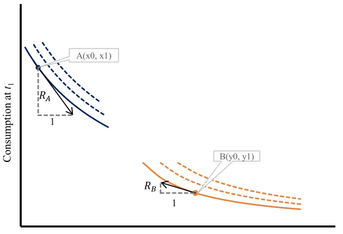
If the two players can borrow from or lend to each other without transaction costs, do they want to reschedule their consumption by borrowing or lending? To answer this question, a key concept is the marginal rate of intertemporal substitution (Frank, 2008, pp.158). The marginal rate of intertemporal substitution (MRIS) is the number of units of consumption in the future (e.g., t1) one would be just willing to exchange for 1 unit of consumption at present (i.e., t0). Mathematically, it is the absolute value of the slope of the intertemporal indifference curve at a given point. As shown in Figure 1.1, at the endowment, player A’s MRIS is RA, which means that
player A is willing to borrow 1 unit for consumption at t0, at the cost of R units of consumption at t1 as long as R < RA. Similarly, player B’s MRIS at the initial
endowment is RB, which means that B is willing to lend 1 unit at t0 as long as she can
get a return of R units at t1 if R > RB. Without the loss of generality, suppose RA > RB.
Then player A and player B can reach an agreement on the borrowing-lending scheme with the intertemporal substitution rate R, as long as R satisfies RB < R < RA. That is,
player A borrows 1 unit from player B at t0 and pay back R units at t1. After this lending-borrowing scheme is arranged to be implemented, player A’s expected consumption at t0 increases to (x0 + 1) and his expected consumption at t1 decreases to (x1 – R). By contrast, player B’s expected consumption at t0 decreases to (y0 – 1) and her expected consumption at t1 increases to (y1 + R).
3 Note that the incomes in Fisher’s (1930) terminology is not necessarily monetary outcomes. They are
Figure 1.1. Indifference curves and marginal rates of intertemporal substitution (RA
and RB) of the two players at their initial endowments. Both players are willing to
trade with each other at certain rate (to reach a better indifference curve) until their marginal rates of intertemporal substitution converge.
The changes to their expected streams of consumption should influence their MRIS. Specifically, player A’s MRIS will decrease and player B’s MRIS will increase. Thus, the difference between the two players’ MRIS becomes smaller. This lending-borrowing scheme will iteratively continue, as long as player A’s MRIS is still larger than player B’s, until their marginal rates of intertemporal substitution converge (RA* = RB*), reaching a stable market equilibrium. The converging MRIS becomes the intertemporal substitution rate, R*, in the market equilibrium ( *
1 0
R = RA* = RB*). In other words, the resulting interest rate in the market is indeed jointly determined by the time preferences of the players in the market.
The illustration above can be generalised to situations where there are any number of players in the market (Fisher, 1930). Importantly, when the number of players is large enough, each player becomes negligible in the market, which means that an individual player's time preference of consumption will have a negligible effect on the interest rate at the market equilibrium. This lays the basis for the analysis of individuals’ optimal intertemporal allocation of consumption and rational
A(x0, x1)
B(y0, y1)
1
𝑅𝐴
𝑅𝐵
1
Consumption at t0
C
onsum
pt
ion
at
CHAPTER 1 INTRODUCTION
6 intertemporal choice between different bundles of resources, which are the focus of Sections 1.1.2 and 1.1.3 respectively.
1.1.2 Intertemporal allocation of consumption
In a market where there are a very large number of players, each player will
have access to a stable per-period interest rate of r0 1 (where r0 1 =
*
1 0
R -1) between
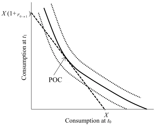
periods t0 and t1, where R*0 1 is the marginal rate of intertemporal substitution (MRIS) between t0 and t1 in the market equilibrium. Thus, with a bundle of resources, one could allocate any amount to each point of time along the dashed-straight budget line as shown in Figure 1.2. Intuitively, individuals’ allocation depends on how differently they value the consumptions at the two periods. Suppose someone only care about her consumption at t0. She will allocate all the resources (i.e., X) to consumption at t0. By contrast, if someone only care about the consumption at t1, she will allocate all the resources (i.e., X(1+r0 1) or X R*0 1) to consumption at t1. However, most people are
not so extreme and usually prefer to spread their consumption over time, which is also the crucial assumption in Fisher’s (1930) framework.4 In other words, when the consumption concentrates on only one period, they are willing to sacrifice a large sum of consumption from that period for a small sum of consumption at the other period. Thus, their indifference curve will be convex as shown in Figure 1.2. Correspondingly, the best indifference curve that they can attain (representing the maximum utility from consumption) is the one that the budget constraint line is tangent to. In other words, people should make their allocation decisions according to the only point of contact (POC) between the curve and the budget constraint line. Any indifference curve that is above (or better than) this indifference curve is unattainable with this budget constraint line.
Figure 1.2. The optimal allocation of consumption to the two periods.
Because of the convexity of the indifference curve, the marginal rate of intertemporal substitution (MRIS) between the two periods depends on the allocation of consumptions of the resources to the two periods. Accordingly, the actual observed
intertemporal preference or MRIS is variable, contingent on the pattern of background consumptions the individual is endowed with. For example, if someone has a large sum of consumption at t0, but a small one at t1, she is probably willing to sacrifice a large sum at t0 in exchange for a much smaller sum at t1. Fisher (1930) regarded pure time preference as the MRIS of the indifference curve when the allocations to the two periods are equal. Defined in this way, Fisher’s (1930) pure time preference for consumption is often not observable and is different from the observed time preference researchers’ observation in the field or experiments.
1.1.3 Intertemporal choice
Researchers are particularly interested in intertemporal choice when two or more options are offered. According to Fisher (1930), in a perfectly competitive capital market, options can be evaluated and compared according to the net present value (NPV). In the NPV model, a stream of incomes can be evaluated by being translated into an equivalent value at present.5 For example, the NPV of the stream of
5 Although the present time point is routinely used as the reference point, it does not matter if a future
time point is used to calculate the equivalent value.
C
onsum
pt
ion a
t
t1
Consumption at t0
X (1+ )
POC
CHAPTER 1 INTRODUCTION
8
x0 at t0 (the present) and x1 at t1 (a future point) can be represented by
1 0 1 0
1 r x x
NPV , where r0 1 is the per-period interest rate between t0 and t1.
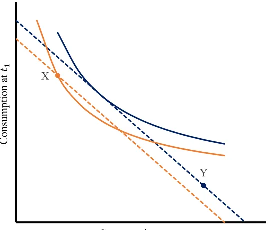
[image:22.595.186.455.373.603.2]It is not difficult to derive that people should choose the option that maximise the net present value in a market with costless, stable and accessible borrowing and lending opportunities, regardless of individuals’ time preference for consumption, because the option with the highest net present value offer a dominant budget constraint line. Take the choice between option X and Y in Figure 1.3 for example. Although Option X is preferred to Option Y at their initial endowments (according to the orange indifference curve), the budget constraint offered by Option X is dominated by that offered by Option Y (according to the dashed budget constraint lines). So, with the given interest rate in the market, decision makers should choose Y instead of X, because Y offers a better net present value or budget constraint than A does and thus attains better indifference curves (see the blue indifference curve).
Figure 1.3. The budget constraint lines of two options with different net present values. Option X is preferred to Option Y at their initial endowments, but the budget constraint line from Option Y (blue dashed) dominates the counterpart from Option X (orange dashed) according to the interest rate in the market.
Y X
Consumption at 𝑡0
C
onsum
pt
ion
The NPV model can generalise to multiple periods with the inter-period intervals of the same length. Individuals’ optimal choice is the option that maximise the NPV according to the interest rates available in the market:
T t t t T t t t r x x t d x x NPV
1 1 1
0 1 0 0 1 1 ) ( ,
where
x
t is the amount of resources (often money) available at time t,d
0 t(
)
is thediscount function for the interval between the present (i.e., a delay of 0) and time t,
1
r
(τ ≥1) is the per-period interest rate over the interval between two consecutiveperiods τ-1 and τ. Note this analysis uses discrete time rather than continuous time.
1.1.4 Forms of discount functions
In this section, I discuss the forms of discount functions in both the NPV model and the DU model over multiple periods.
The net present value (NPV) model. Fisher (1930) did not provide a general
form of the discount function. However, research and practice in economics and
finance often assumes constant interest rate over time, i.e.,
r
1 = r for allτ ≥1 (e.g., Brealey, Myers, & Allen, 2012; Frank, 2008, p.156; Hey, 2003), although constant interest rate does not have a strict normative basis (Fisher, 1930). Thus, the net present value (NPV) model becomes,T t t t r x NPV 0 1 1 ,
where r is the constant per-period interest rate available in the market. The
corresponding per-period discount factor is
r
1
1 and the per-period discount rate
is 1 - δ.6
The discounted utility (DU) model. In terms of the intertemporal allocation
of consumption, Paul Samuelson’s (1937) discounted utility (DU) model has been long regarded as the normative model:
6 Keynes (1936) discussed commodity-specific interest rates when the exchange rate between
CHAPTER 1 INTRODUCTION 10 T t t c t r c u U 0 1 1 ) ( ,
where
r
c is the constant per-period personal interest rate for consumption. Thecorresponding per-period discount factor is
c c
r 1
1
and per-period discount rate is
1 - δc.
Strotz (1955) shows that a constant interest rate for consumption in the DU model is necessary to achieve time-consistent allocation of consumption over time.7 Otherwise, people would keep changing the allocation of consumption over the passage of time. For example, as shown in Figure 1.4, a decreasingly impatient person gives special weights to temporally proximal selves and over-consume the resources and thus leave less for future selves. When future selves come closer in time, one of the “future” selves become the “present” one, she is going to re-evaluate and again give special weights to the present and temporally close selves and over-consume. When this iterative process happens for multiple selves, the far-future selves will get almost nothing. Koopmans (1960) provides a formal axiomatization for the constant interest rate in the discounted utility model.
Figure 1.4. Time-inconsistent allocations of consumption over time (Strotz, 1955).
7 Note that this is not incongruent with Fisher’s (1930) argument that the degree of impatience should be influenced by background consumption, because Fisher’s (1930) observed time preference is defined on the objective amounts of consumption but the time preference (or discount rate) in Samuelson’s
In terms of the interest rate for different goods, Samuelson (1937) does not
discuss whether there is a single interest rate
r
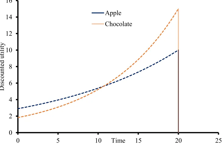
c governing all different types of goods [image:25.595.136.502.396.632.2]or there are good-specific interest rates. However, I argue that a unity of the interest rate for the consumption of different goods should hold as a postulate for the DU model. Otherwise, a cross-modal intertemporal choice could result in dynamic inconsistency in intertemporal choice (see Read & van Leeuwen, 1998; Read, Loewenstein, & Kalyanaraman, 1999).8 For example, suppose an apple is worth 10 utils, a chocolate is worth 15 utils and the discount rate for the utility of consuming a chocolate is larger than the discount rate for the utility from consuming an apple. Considering a choice of a chocolate and an apple available at the time point T20 (see Figure 1.5). At T0, the apple is preferred to the chocolate but, the preference is reversed when the time of decision comes closer to the time of consumption. For example, at T15, the chocolate is preferred to the apple.
Figure 1.5. Time-inconsistent choice between different goods when discount rates differ across goods.
8 Another way of interpreting the time-inconsistent preference of the apple and the chocolate is that the
consumption of the chocolate is for immediate enjoyment but the consumption of the apple is for future health. However, this alternative explanation does defect the illustrative power of different discount rates for the consumption of different goods.
0 2 4 6 8 10 12 14 16
0 5 10 15 20 25
D
isc
ount
ed
ut
il
it
y
CHAPTER 1 INTRODUCTION
12
Differences between the NPV and the DU models. There are two salient
distinctions between the NPV model and the DU model. First, The NPV model involves the discount of the market value of bundles of resources, as long as they can be traded in the market, but the DU model involves the discount of the utility from consumption of resources. Second, the interest rate in the NPV model is the rate available in the market, while the interest rate in the DU model is a personal interest rate of utility from consumption and is unrelated to the interest rate in the market. Put in another way, the interest rate in the NPV model is universal to all participants in the same market but the interest rate in the DU model could be person-specific. However, many studies on intertemporal choice failed to make a distinction between them and thus making mistaken claims.
The use of the NPV or DU model as the normative model depends on the objective of a study. If a study is to investigate whether people are excessive discounters compared with the interest rate available in the market, the NPV model should be used as the normative standard. However, it is important to note that when using NPV, we assume that the incomes or goods are tradable in a market (e.g., money, food). If a study focuses on the consumption of incomes and goods, which is always the case in the literature, DU should be used as the normative standard. Researchers could compare people’s discount rates from the DU model. However, we should be cautious about the assumptions we make for the utility function. For convenience and simplicity, the utility of consumption is always deemed equivalent to the raw amount of consumption (e.g., Charlton & Fantino, 2008; Estle et al., 2007; Odum, Baumann, & Rimington, 2006; Odum & Rainaud, 2003; Tsukayama & Duckworth, 2010; Ubfal, 2016). This is problematic for many cases due to reasons such as satiation, which will be discussed later.
1.1.5 Optimal choice when borrowing and lending rates differ
Cubitt and Read (2007) analysed the situation where the borrowing and the saving interest rates were different (see also Coller & Williams, 1999). Suppose the borrowing rate is 20% per annum and the saving rate is 1% per annum. Intuitively, there would be two different interest rates to calculate the net present value when choosing between two or more options. If the calculation of net present values according to both rates favour the same option, then people should choose the option with the highest net present value. However, if the net present value according to the two interest rates favour different options, then decision makers’ optimal choice depends on the financial circumstances they are facing. If decision makers are saving at the rate of 1% per annum, they should choose the option that is favoured by the net present values according the annual rate of 1%. By contrast, if they are borrowing at the rate of 20%, she should choose the option that is favoured by the net present values according to the annual rate of 20%.
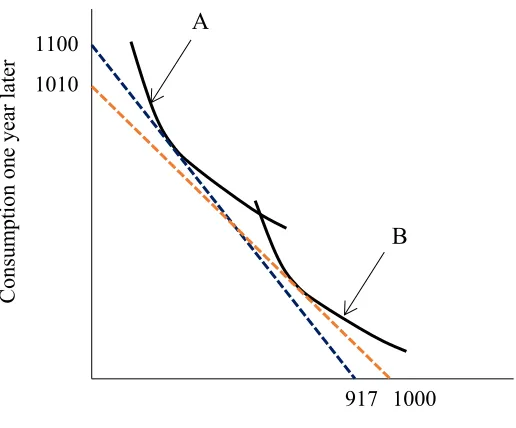
Figure 1.6. Optimal choice when borrowing and lending rates differ. The orange dashed line is the budget constraint from receiving $1000 today (SS), with the saving interest rate of 1% per annum. The blue dashed line is the budget constraint from receiving $1100, with the borrowing interest rate of 20% per annum (LL).
If the net present value according to the two interest rates favour different options and if the decision maker has neither saving nor debt, the NPV model no longer offer a conclusive answer. Consider, for example, a choice between receiving
B
C
onsum
pt
ion on
e ye
ar
lat
er
Consumption now
A
917 1000
CHAPTER 1 INTRODUCTION
14 $1000 now (referred to as SS) and receiving $1100 in one year (referred to as LL), implying an interest rate of 10% per annum. Suppose the two options are only allocated for consumption at two periods: now and in-one-year. As shown in Figure 1.6, on one extreme, if the SS option is all spent now, the amount for consumption now is $1000. On the other extreme, the SS option can be all saved with an annual rate of 1% and thus the amount for consumption in one year is $1010. It can also be partly spent now and partly saved for one-year later. So the budget constraint line from the SS option is shown as the orange dashed line in Figure 1.6. Likewise, the LL option
can be all spent in one year ($1100), all spent now (borrowing 1$110020% = $917 now for
consumption and paying back $1100 in one year), or partly spent now and partly spent in one year. So the budget constraint line from the LL option is shown as the blue dashed line in Figure 1.6. Importantly the budget constraint lines offered by the two options intersect at certain point. Thus, decision makers’ optimal choice will depend on their personal intertemporal preferences for consumption and should choose the option that bring them to the best indifference curve, rather than the interest rates in the market (Cubitt & Read, 2007). For example, as shown in Figure 1.6, A should choose the LL option because it is the LL option that brings her to her best attainable indifference curve while, for the same reason, B should choose the SS option.
1.1.6 Interim summary
With both the NPV model and the DU model, we can reconsider the diverse claims made in the literature. First, for tradable goods (in a perfectly competitive capital market), the NPV model, which has an interest rate related to the interest rate available in the market, should be the normative model to evaluate the choice among two or more options. With the NPV model, the interest rate elicited from laboratory experiments can be compared with the prevailing interest rate in the market. Second, the DU model, which endorses individual-specific discount rate, is the normative model for intertemporal allocation of consumption for the sake of time consistency. This interest rate is incomparable with the prevailing interest rate in the market. Third, for each individual person, the discount rate in the DU model should be the same for different goods for the sake of time consistency.
1.2 Empirical Findings
These studies, with few exceptions, have shown substantial departure from the normative predictions.
1.2.1 Monetary outcomes
Among all, many studies on intertemporal choice used monetary outcomes. The most frequently used tasks are choices between smaller-sooner (SS) and larger-later (LL) monetary options. Researchers always infer the discount rate from decision makers’ choice in SS-LL questions. For example, if someone choose SS in a choice between receiving $100 today (SS) or receiving $150 in a year (LL), the choice suggests that the decision maker requires an interest rate over 50% per annum. Some also used choices between sequences of monetary outcomes. Because of the liquidity of money, it is reckoned that people can reschedule the consumption of the money by borrowing from and saving in the market. Thus the net present value (NPV) model is considered the economic standard for intertemporal choice of monetary outcomes. In this section, I review findings from the studies using monetary outcomes.
Excessive discounting. Excessive discounting refers to that the discount rates
elicited from intertemporal choice between monetary outcomes are excessively higher than what is available in the market (Frederick et al., 2002; Read et al., 2005). As discussed earlier, the interest rate at which one can get from saving in banks is relatively low. The interest rates people can earn from other investments (e.g., securities, bonds and stocks) are generally not be too high either. The interest rates that one need to pay for loans are higher, but are mostly lower than 30% per annum in the UK or other western countries. However, in laboratory or field experiments, people always require interest rates higher than 100% per annum (see Frederick et al., 2002 for a review). For example, many people would prefer receiving $100 now to receiving $250 in one year.
Sign effect. The sign effect is that people discount more steeply for delayed
CHAPTER 1 INTRODUCTION
16
Absolute magnitude effect. The absolute magnitude effect is that implied
discount rates decrease with the magnitude of the outcome (Loewenstein and Prelec 1992). For example, someone indifferent between $200 in one year and $100 today would probably prefer $2,000 in one year to $1,000 today. It is one of the most robust phenomena in intertemporal choice and has been corroborated in a wide range of studies (e.g., Baker, Johnson, & Bickel, 2003; Benhabib, Bisin, & Schotter, 2010; Benzion, Rapoport, & Yagil, 1989; Green, Fristoe, & Myerson, 1994; Holcomb & Nelson, 1992; Petry, 2001; Thaler, 1981).
Delay effect. The delay effect is that people require higher interest rate for
short delays than for long delays (Thaler, 1981). For example, someone indifferent between $100 today and $225 in two years (implying an interest rate of 50% per annum) would probably prefer $100 today to $150 in one year (implying an interest rate over 50% per annum). Concerning the delay effect, there are two different explanations. One is decreasing impatience and the other is subadditive discounting (Read, 2001). See further discussion of the two effects below.
Non-constant discounting. Non-constant discounting includes decreasing
impatience and increasing impatience. In some literature, decreasing impatience is also known as the common difference effect, which means that the interest rate over an interval decreases as the delay to the onset of the interval increases (Loewenstein & Prelec, 1992). For example, someone indifferent between $200 in one year and $100 today would probably prefer $200 in two years to $100 in one year. This effect has been corroborated in several studies (e.g., Green et al., 1994; Green, Myerson, & Macaux, 2005; Holt Green, Myerson, & Estle, 2008; Keren & Roelofsma, 1995; Kirby & Herrnstein, 1995; Scholten & Read, 2006). However, some others have found evidence for increasing impatience that the discount rate over an interval increase with the onset of the interval (e.g. Holcomb & Nelson, 1992; Read et al., 2005; Sayman & Öncüler, 2009; Attema et al., 2010).
Non-additive discounting. Non-additive discounting is that the discounting
over an interval depends on whether it is divided into sub-intervals or is kept undivided. Two patterns of non-additivity have been observed: subadditivity and superadditivity.
someone indifferent between $100 now and $150 in six months and indifferent between $150 in six months and $200 in one year would prefer $200 in one year to $100 today. Superadditivity is the reversal of subadditivity, in that implied discount rates are higher over an undivided interval than over an interval that is divided into subintervals (Scholten & Read, 2006; 2010; Scholten et al., 2014).
Sequence effects. Intertemporal choices between sequences of positive
outcomes have been shown to be different from those between single-dated outcomes. Most compellingly, negative time preference, which means a preference for a positive outcome to take place later rather than earlier, has been frequently observed when participants choose between intertemporal sequences (Loewenstein & Prelec, 1993; Loewenstein & Sicherman, 1991; Read & Powell, 2002), but is rarely observed when they are asked to choose between two single-dated outcomes.
Framing effects. The literature has documented diverse framing effects
CHAPTER 1 INTRODUCTION
18
1.2.2 Non-monetary outcomes
Although a majority of studies used monetary outcomes for research into intertemporal choice, there is still a significant proportion of studies using other commodities as outcomes, such as food, drinks and other consumable goods.
Domain-specific discounting. Most of the studies on the discounting of
consumable commodities made a comparison between the interest rates of consumable commodities and that of monetary outcomes. The results often suggested that directly consumable goods (e.g., alcohol, food, CDs and DVDs) are discounted more steeply than money (e.g., Charlton & Fantino, 2008; Estle et al., 2007; Odum, Baumann, & Rimington, 2006; Odum & Rainaud, 2003; Tsukayama & Duckworth, 2010; Ubfal, 2016). There are some exceptions though. Hardisty and Weber (2009) found that the discount of monetary outcomes, (public) environmental goods and health was similar to each other. Chapman (1996b) found that the discount rate for health was always higher than that for money.
While there is always a gap between discounting of money and consumable commodities, individuals’ discount of money and consumable commodities are still correlated. Reuben, Sapienza and Zingales (2010) found that the discount rates for money and chocolates were moderately correlated. Odum (2011) showed that the discount rate for money was highly correlated with the discount rates for a variety of consumable commodities (i.e., food, heroin and cigarettes). Ubfal (2016) also found that high degrees of correlation among discount rates of a variety of goods including money, meat and sugar. Tsukayama and Duckworth (2010) showed that the correlation between discount rates of money and that of consumable goods were lower than the correlation of discount rates among different consumable goods, drawing a second line between directly consumable goods and money.
A surprising observation in these studies mentioned above is that when the discount rates of different goods were compared, none of them used the DU model to estimate individual discount rates. Instead, discount rates are usually measured with the quasi-hyperbolic discounting model (Laibson, 1997), the hyperbolic discount model (Mazur, 1987) and/or a model-free estimation called Area Under the Curve (AUC: Myerson, Green, & Warusawitharana, 2001).
Utility function. Although many studies claimed to identify domain-specific
linear function of amount of consumption, even for food (see Kirby and Santiesteban, 2003 for an exception). A closely related issue to the utility function is satiation of consumptions (Read et al., in press). For example, someone having two pizzas for oneself to eat will not be twice as happy as when she has only one pizza to eat. So, an important empirical concern is the elicitation of utility function.
Measuring the curvature of the utility function is a difficulty. Different approaches have been proposed. Andersen et al., (2008) used the method of double elicitation. With monetary outcomes, Andersen et al. (2008) elicited the curvature of the utility function for money from risky choice and applied the utility function from risky choice to intertemporal choice. Some others have attempted to elicit time preference by avoiding the curvature of the utility function through their experimental designs (Attema et al., 2010; Chapman, 1996b; Laury, McInnes, & Swarthout, 2012). Although the technical solutions of these designs differ from one another, they share the same intuition that the amounts of the outcomes in SS and LL are kept constant across items. However, these methods were applied to monetary outcomes only. Further research should pay more attention to the curvature of the utility function.
1.3 Causes of Departures from the Normative Models
Empirical tests of intertemporal choice of money or non-monetary goods have shown substantial departures from the predictions by the NPV model or the DU model. Various causes have been proposed to explain the departures including both environmental factors and cognitive limitations.
1.3.1 Market imperfection and complication
CHAPTER 1 INTRODUCTION
20 Concerning the variability of discount rates for different commodities, Keynes (1936) points out that the exchange rate between commodities is not constant across time. Indeed, even the exchange rate between two currencies, such as sterling pounds and dollars, keeps changing over time. Other important factors that influence commodity-specific interest rates include the yield, the carrying cost and the liquidity premium (Keynes, 1936; Read et al., in press). The yield means the owner’s benefit from the use of a good, especially when the value of the good is not much reduced after the use. The yield is especially applicable to durable goods, such as a house. The owner of the house can use the house as accommodation, but the value of the house in the market is more or less maintained. The carrying cost refers to the cost incurred during the good is held, such as storage, obsolescence, spoilage and wastage. A good example is fresh vegetables sold in supermarkets. The liquidity premium refers to the convenience of a good to be exchangeable to other goods with the identical market value. Among all, money, as the common currency, probably has the highest liquidity premium. For example, one can buy candies or shop groceries with money. But it is inconvenient to exchange candies for groceries or vice versa.
1.3.2 Background consumption
While background consumption is one of most important determinants of the observed time preference in Fisher’s (1930) framework, it often dismissed in the vast number of studies investigating individual differences in intertemporal preference (e.g., Dohmen, et al., 2010; Enzler et al., 2014; Shamosh et al., 2008) and discounting of different goods (e.g., Augenblick et al., 2012; Chapman, 1996b; Estle et al., 2007). It is especially problematic when the curvature of the utility function (in the DU model) is not taken into consideration. For example, Noor (2009) used the curvature of the utility function induced by background consumption to explain hyperbolic discounting on raw amounts.
Moreover, it is almost indistinguishable between the utility function and the discount rate in the DU model (Read et al., in press). For example, when someone is highly desired for an immediate consumption at the cost of the consumption later of a much larger amount, it could be attributed to a high discount rate but it could be equivalently attributed to a disproportionately large utility from the current consumption.
function. However, as discussed earlier, this pure time preference is defined as the marginal rate of intertemporal substitution only when the background consumption is equal at different time periods. Thus it is often unobservable and is unlikely to overcome the obstacles from background consumption either.
1.3.3 Uncertainty associated with delayed offers
Many people may be concerned with the uncertainty of the delayed outcome when faced with a choice between an immediately available and a delayed outcome (Epper, Fehr-Duda, & Bruhin, 2011; Fisher, 1930). Sozou (1998) shows that a hyperbolic discount function can arise from the (constant) exponential discounting function if future outcomes are uncertainty. Michaelson et al. (2013) showed that people are more likely to choose the delayed but larger reward when the person who is going to deliver it looks trustworthy than when the person looks untrustworthy, which implies that the delayed option is perceived as risky in the meantime.
Because of the confound of uncertainty, some studies took measures to control the uncertainty of a delayed payment. For example, Andreoni and Sprenger (2012) tried to guarantee the delayed payments using a credit system. In Andersen, Harrison, Lau and Rutstrom (2008), delayed payments to participants were guaranteed by a national Ministry in Denmark and was paid directly into participants’ personal bank accounts.
1.3.4 Subjective perception of delays
Psychophysical accounts suggest that subjective perception of or sensitivity to delays is a source of non-constant discounting. Takahashi (2005) shows that a generalized hyperbolic discount function by Loewenstein and Prelec (1992), which embodies decreasing impatience, can be derived from constant impatience with a decreasingly elastic function for subjective time perception. Experimental studies have supported this view by showing that the subjective perception of delays is nonlinear and that the discounting over the subjective perception of delays tends to be constant (Han &Takahashi, 2012; Zauberman, Kim, Malkoc, & Bettman, 2009). Ebert and Prelec (2007) extended the view of subjective sensitivity to delays to allow for both decreasing and increasing impatience.
1.3.5 Myopia or a lack of self-control
CHAPTER 1 INTRODUCTION
22 and over-consume the resources and thus leave less for future selves. When future selves come closer in time, the “future” selves become the “present” ones and again over-consume. When this iterative process happens for multiple selves, the far-future selves will get almost nothing (Figure 1.4). This lays the foundations of many studies of intertemporal choice in behavioural economics and has been applied to diverse phenomena such as pension scheme (Laibson,1997), credit card borrowing (Meier & Sprenger, 2012), procrastination (O’Donoghue & Rabin, 1999) and addiction (Heyman, 1996).
1.3.6 Cognitive inertia
Lastly, but probably most importantly for the thesis, cognitive inertia could be a key drive behind intertemporal choice. As shown by Frederick (2005), a simple Cognitive Reflection Test (CRT) consisting of three items is a prominent predictor of intertemporal discounting. CRT is a psychological battery that assesses to what degree one is likely to use intuitive heuristics or deliberative thinking, analogous to dual-systems (Sloman, 1996; Kahneman and Frederick, 2002). Based on CRT, those with high cognitive reflection are much less impatient than those with low cognitive reflection in intertemporal choice of monetary outcomes.
Various framing effects are also strong evidence for the key role of cognitive inertia in intertemporal choice. These effects suggest that most decision makers not only skip optimising, but also make decisions in respect to many normatively irrelevant information (see framing effects in Section 1.2.1, pp. 17). A good example is from Read et al. (2013), their participants exhibited much less impatience when the intertemporal choice between monetary outcomes was described as an investment, while the normative account suggest that people are always aware of investment opportunities. It is these framing effects that call for a more coherent understanding of the psychology of intertemporal choice.
1.4 Cognitive Processes in Intertemporal Choice
environmental features relating to the making of decisions, even rational individual behaviour could depart from the prediction of the model. Second, various framing effects suggest that individuals show inconsistent preferences when normatively equivalent decisions (see framing effects in Section 1.2.1, pp. 17). Those effects are frequently explained by different cognitive processes invoked by different framing, highlighting the importance of studying cognitive processes in intertemporal choice (e.g., Cubitt, McDonald, & Read, 2017; Read et al., 2016; Weber et al., 2007). Below, I briefly introduce several important cognitive processes that could govern individual intertemporal choice, which are also the focus of the following chapters in the thesis.
1.4.1 Evaluation rule
One of the fundamental questions regarding the cognitive processes of intertemporal choice, as well as other types of value-based decision making, is how information of the choice is processed and evaluated. There are mainly two different evaluation rules in intertemporal choice: alternative-based and attribute-based rules (see Scholten et al., 2014; Dai & Busemeyer, 2014).9 According to the alternative-based rule, options are evaluated and assigned values independently. The option with the highest assigned value is chosen. By contrast, the attribute-based rule assumes that options are directly compared along the time and outcome attributes respectively, and the option favoured by these comparisons is chosen (e.g., Gonzalez-Vallejo, 2002; Tversky, 1972).
Two strands of evidence could shed light on the comparisons of different evaluation rules. First, eye-tracking studies offer the process-level evidence on whether decision is made by alternative-wise computation or attribute-wise comparison. For example, Arieli, Ben-Ami and Rubinstein (2011) found that participants make intra-attribute eye movements much more often than intra-option eye movements. Second, different evaluation rules are written in models and thus the descriptive accuracy of the models with different evaluation rules behind can be quantitatively compared with each other (e.g., Scholten et al., 2014; Dai & Busemeyer, 2014).
9 A third evaluation rule was used in Scholten and Read’s (2006) interval discounting model. See further
CHAPTER 1 INTRODUCTION
24
1.4.2 Attention
Attention allocation matters in many value-based decision making, including intertemporal choice. Many studies posit that attention is a key cognitive process that drives value-based preference (e.g., Bhatia, 2014; Bordalo, Gennaioli, & Shleifer, 2012; Kőszegi & Szeidl, 2013; Read et al., 2013; Tsetsos, Chater, & Usher, 2012; Tversky, Sattath, & Slovic, 1988; see Weber & Johnson, 2009 for a review). A few studies have directly tested the relationship between attention and food choice (Armel, Beaumel, & Rangel, 2008; Krajbich, Armel, & Rangel, 2010), risky choice (e.g., Fiedler & Glőckner, 2012; Stewart, Hermens, & Matthews, 2016) and intertemporal choice (e.g., Fisher & Rangel, 2014; Franco-Watkins, Mattson, & Jackson, 2016). A better understand of the attention effects on intertemporal choice is a key step towards the understanding of cognitive processes of intertemporal choice.
1.4.3 Background contrast
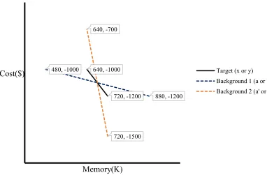
Background contrast is another important cognitive factor that have been found to play an important role in value-based decision making (Simonson & Tversky, 1992). This effect has been very well-established in a wide range of studies (Ebert & Prelec, 2007; Priester, Dholakia, & Fleming, 2004; Simonson & Tversky, 1992; Vlaev & Chater, 2006; 2007; Walasek & Stewart, 2015). In their seminal work, Simonson and Tversky (1992) showed that participants’ tradeoff between two attributes (e.g., the price and the quality of a personal computer) was strongly influenced by the preceding tradeoff they have been exposed to, regardless of their choices in the preceding tradeoff.10 For example, as shown in Figure 1.7, in a choice between paying $1200 for a computer with 720K memory (Option x) or paying $1000 for a computer with 640K memory (Option y), participants were more likely to choose x when they had been previously exposed to a choice between paying $1200 for a computer with 880K memory (Option a) or paying $1000 for a computer with 480K memory (Option b) than when they had been previously exposed to a choice between paying $1500 for a computer with 720K memory (Option a’) or paying $700 for a computer with 640K memory (Option b’).
10 A closely related effect to the background contrast effect is the prospect relativity effect (e.g., Stewart,
Figure 1.7. A graphical illustration of Simonson and Tversky’s (1992) study on the background contrast effect.
1.5 Overview of the Following Chapters
The thesis is aimed at a better understanding of the cognitive processes in intertemporal choice. Three separate empirical studies are reported in Chapters 2-4, investigating various cognitive processes including evaluation rules, attention, and background contrast. Chapter 5 further summarises the results from the empirical studies and discusses the implications on theory development of intertemporal choice. The study in Chapter 2 makes a comprehensive model comparison in intertemporal choice. The literature has documented a wide array of intertemporal choice models. However, existing studies that quantitatively compare intertemporal choice models often lend support to different models. Several limitations make it difficult to compare the results from different studies. This comprehensive model comparison attempts to address or, at least, alleviate three limitations: Model selectivity, stochastic-specification selectivity and stimulus diversity. The results lend strong support to attribute-based models, especially the family of the tradeoff model. There is also an interaction between models and stochastic specifications on model performance, highlighting the importance of stochastic specification in intertemporal choice modelling.
720, -1200 640, -1000
880, -1200 480, -1000
720, -1500 640, -700
Cost($)
Memory(K)