Validation of geometry modelling approaches for offshore gas dispersion simulations

warwick.ac.uk/lib-publications

Ahmed, A., Bengherbia, T., Zhvansky, R., Ferrara, G., Wen, Jennifer X. and Stocks, N. G.. (2016) Validation of geometry modelling approaches for offshore gas dispersion simulations. Journal of Loss Prevention in the Process Industries .

Permanent WRAP URL:

http://wrap.warwick.ac.uk/81314

Copyright and reuse:

The Warwick Research Archive Portal (WRAP) makes this work by researchers of the University of Warwick available open access under the following conditions. Copyright © and all moral rights to the version of the paper presented here belong to the individual author(s) and/or other copyright owners. To the extent reasonable and practicable the material made available in WRAP has been checked for eligibility before being made available.

Copies of full items can be used for personal research or study, educational, or not-for-profit purposes without prior permission or charge. Provided that the authors, title and full bibliographic details are credited, a hyperlink and/or URL is given for the original metadata page and the content is not changed in any way.

Publisher’s statement:

© 2016, Elsevier. Licensed under the Creative Commons Attribution-NonCommercial-NoDerivatives 4.0 International http://creativecommons.org/licenses/by-nc-nd/4.0/

A note on versions:

The version presented here may differ from the published version or, version of record, if you wish to cite this item you are advised to consult the publisher’s version. Please see the ‘permanent WRAP url’ above for details on accessing the published version and note that access may require a subscription.

Validation of geometry modelling approaches for

offshore gas dispersion simulations

I. Ahmeda,b,∗, T. Bengherbiaa, R. Zhvanskya, G. Ferraraa, J. X. Wenb, N. G. Stocksb

a_{DNV GL, London, UK}

b_{Warwick FIRE, School of Engineering, University of Warwick, Coventry, UK}

Abstract

Computational Fluid Dynamics (CFD) codes are widely used for gas dis-persion studies on offshore installations. The majority of these codes use single-block Cartesian grids with the porosity/distributed-resistance (PDR) approach to model small geometric details. Computational cost of this ap-proach is low since small-scale obstacles are not resolved on the computa-tional mesh. However, there are some uncertainties regarding this approach, especially in terms of grid dependency and turbulence generated from com-plex objects. An alternative approach, which can be implemented in general-purpose CFD codes, is to use body-fitted grids for medium to large-scale ob-jects whilst combining multiple small-scale obstacles in close proximity and using porous media models to represent blockage effects. This approach is validated in this study, by comparing numerical predictions with large-scale gas dispersion experiments carried out in DNV GLs Spadeadam test site. Gas concentrations and gas cloud volumes obtained from simulations are compared with measurements. These simulations are performed using the commercially available ANSYS CFX, which is a general-purpose CFD code. For comparison, further simulations are performed using CFX where small-scale objects are explicitly resolved. The aim of this work is to evaluate the accuracy and efficiency of these different geometry modelling approaches.

Keywords: gas dispersion, geometry modelling, computational fluid dynamics

1. Introduction

Hazardous materials being released into the atmosphere is one of the main causes of accidents in oil and gas installations. The accidental release and subsequent dispersion of flammable gases could cause fires and explosions. Therefore, consequence analysis of gas dispersions is crucial when optimizing the location of gas detectors and to determine the risk of fire and explosion. A number of modelling techniques are used for consequence analysis of accidental gas releases. These include empirical, phenomenological and Com-putational Fluid Dynamics models. Both empirical and phenomenological models can provide an estimate quickly and are widely used in the oil and gas industry. However, these models have a limited range of validity since they cannot capture the effects of obstacles and complex terrains.

In contrast, CFD models solve the equations of fluid mechanics in three-dimensions, thus, enabling the accurate representation of complex geometries that are often found in oil and gas production facilities. This makes CFD the preferred method to study gas dispersion, especially for offshore oil and gas installations.

However, the use of CFD is not without its own challenges. One of the major drawbacks of CFD is the time taken to generate the computational mesh required for the simulation. The computational and mesh size and, hence, the cost of such simulations will become prohibitively expensive if one were to resolve all geometrical obstacles (pipes, instrumentation, equipment etc.).

media.

Fothergill et al. [3] estimated the drag on the flow through the porous region used to represent small-scale geometries. This estimate was made by calculating the drag due to each object and obtaining a sum of the over-all resistance. This method was implemented in another commercial CFD package called CFX. They compared their results with EXSIM CFD code that uses PDR method and showed that the turbulent kinetic energy and turbulent eddy dissipation predicted by CFX was much lower than EXSIM. The porous model they used simply reduced the volume of free flow and provided extra resistance, but did not generate turbulence. They proposed the inclusion of additional source terms in the turbulence kinetic energy and dissipation equations to account for turbulence generation by the obstacles.

Savvides et al. [4] used FLUENT CFD code to simulate large-scale dis-persion of fuel in an offshore module, where small-scale objects were treated as porous media, with the coefficients based on BP data. They showed that this approach can predict gas dispersion with good accuracy. Ivings et al. [5] simulated an under-expanded jet impinging on an array of pipes. In the porous approach, momentum sink terms were included in the fluid flow equations to account for the effect of pipes. They also included turbulence source terms based on the explosion model by Hjertager et al. [6]. Their simulations showed that resolving the objects on the grid did not offer any significant advantages over the porosity based approach.

The main aim of this work is to carry out a validation study of the porosity approach by comparing with large-scale dispersion experiments carried out at DNV GLs Spadeadam test site. In addition comparison is also made with simulations where the small-scale objects are full resolved. The commercial, general purpose CFD package, ANSYS CFX version 15.0 is used for the simulations carried out in this work.

2. Experimental test cases

Gas concentration was monitored at 50 locations inside the test rig using oxygen sensors. The gas concentrations reported by the experiments were when steady-state conditions have been reached. Meteorological conditions such as the ambient wind speed (horizontal component) and direction were measured using an ultrasonic anemometer, mounted at 20 m above ground.

Twenty-three gas dispersion experiments were carried out using two con-finement configurations. In this work, only one concon-finement configuration is considered, in which one side of the module is open and the remaining 3 sides and roof of the module is closed. Two leak scenarios are considered, which are given in Table 1.

Table 1: Two test cases simulated in this work; includes leak properties and atmospheric conditions during the test.

Test case Leak Leak Leak Orifice Wind Wind

case Location (x, y, z) direction rate (kg/s) diameter (mm) speed (m/s) direction (◦)

16 5.5,6,1.7 +X 2.6 32.5 0.9 3.66

17 5.5,6,1.7 +X 6.9 32.5 4.2 6.97

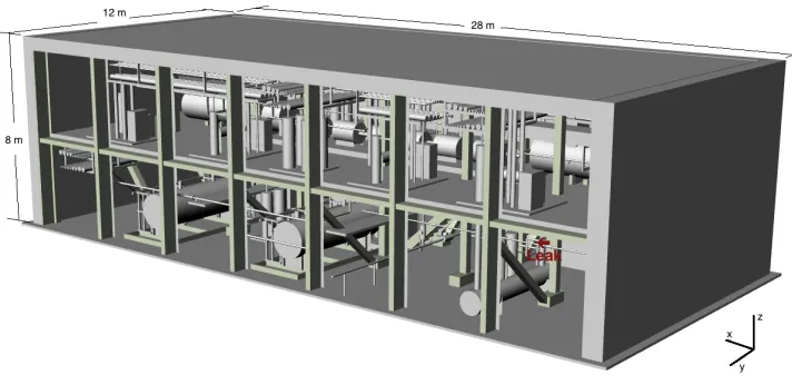
The leak location, direction, orifice diameter are identical; the only differ-ence being the leak rate. The wind speed and wind directions are averaged quantities measured during the experiments. Fig. 1 shows the CAD model of the experimental rig with the location of the leaks marked (the two leaks used in this study are pointing along positive x-direction).

3. Numerical setup

3.1. Governing equations

CFD involves the solution of highly non-linear, coupled partial differen-tial equations. These are the equations of mass conservation, Navier-Stokes (momentum conservation) and energy equations. In addition, in dispersion problems one needs to solve additional transport equations for the gas.

Fig. 1: Experimental rig with dimensions. Location of the leaks are also highlighted in red.

3.2. Turbulence model

Reynolds-averaging the governing equations lead to the famous turbu-lence closure problem, which requires models to close the equations. A num-ber of turbulence models have been developed over the years, the standard k- model being the most popular for gas dispersion studies. It is well known that the standard k- model yields poor results for separated flows, impinge-ment and flows with extra strains [8].

One improvement to the standard k-model is the Renormalization Group (RNG) k-model, which is better suited for separated flows and flows around bluff bodies [8]. Therefore, the RNG k- model is used in this work along with scalable wall functions to model the boundary layer near the walls and the terrain. Note that the default turbulence parameters used in ANSYS CFX v15.0 [9] are used in this work without any modification.

3.3. Geometry and mesh generation

example piping) are combined to form a porous region. This geometry will be referred to as the porous geometry. The cut-off criteria are: any pipe with diameter smaller than 15.24 cm and boxes with cross-sectional area smaller than 232 cm2 _{are treated as small-scale objects.}

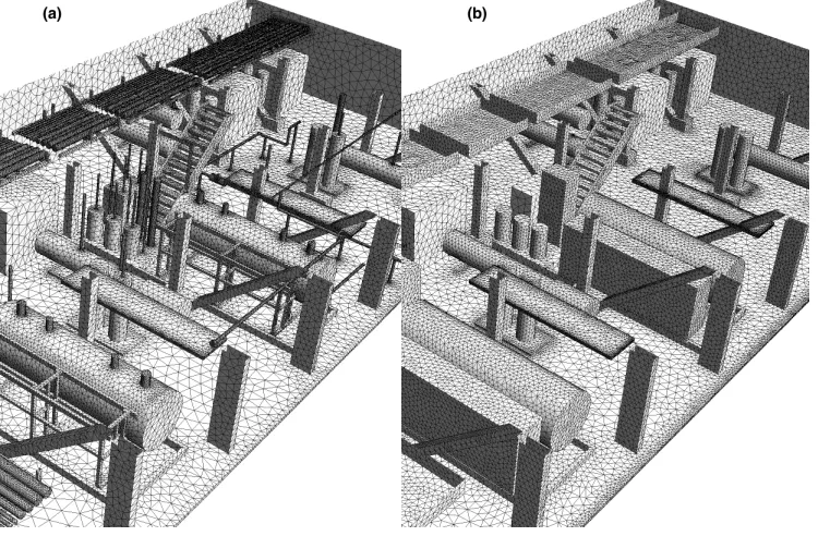
ANSYS ICEM CFD is used to generate the computational meshes for these two geometries. Unstructured tetrahedral mesh generation is used since it is relatively quick to generate a mesh, even for complex geometries. Grid independence studies were performed initially for both geometries to ensure that the results are independent of the grid used. Figures 2(a) and 2(b) respectively show the surface mesh generated for the geometry where all the small-scale objects are resolved and geometry where these small-scale objects are represented using porous regions. Since the leak sizes are different between tests 16 and 17 the meshes generated for these two cases are different as well. The meshes shown in Figure 2 are for test 16. In order to accurately resolve the boundary layers, prism layers are added adjacent to the terrain.

CFX is node based solver, therefore, the number of nodes is the relevant parameter to determine the mesh size. Table 2 shows the mesh sizes for both geometrical representations in each of the two tests. This table shows that the resolved mesh is generally three times larger than the mesh with porous regions.

Table 2: Number of nodes used for the resolved mesh with porous regions.

Test case No. of nodes in resolved mesh No. of nodes porous mesh case (in millions) (in millions)

16 3.8 1.1

17 4.5 1.6

3.4. Porosity generation

For high Reynolds number turbulent flows one could write the momentum source term as [10]

Si =

1

2C2ρ|ui|ui, (1)

where C2 is the inertial pressure loss coefficient and ui is the superficial

velocity solved using CFD. Similarly, the source terms for turbulence kinetic energy, k, and turbulence dissipation rate,, are given respectively as

Sk=

1

2C2Ckρ|ui|

3

, (2)

Sk=ρ

Cmu3/4k3/2−

L , (3)

whereLis the turbulence length scale associated with the porous region and in this work it is taken as 10% of the obstacle length in a given coordinate direction, Ck is a turbulence constant and is generally assumed to be

inde-pendent of the obstacle type [10]. One method of obtaining C2 is to use

the Ergun equation [11], which gives the pressure drop across a packed bed. Using this method C2 can be given by

C2 =

3.5(1−p)

dpp3

, (4)

where p is the porosity and dp is the particle diameter. Porosity was

calcu-lated by determining the volumed blocked by small piping structures in the volume of interest. The directional arrangement of the pipes and small struc-tures means that one cannot assume isotropy for the source terms; instead, different source terms were obtained for the three coordinate directions.

3.5. Initial and boundary conditions

For atmospheric flows, velocity and turbulence profiles need to be defined at the inlet boundaries. The velocity profile by Richards and Hoxey [12] is used in this work, which is given by

U(z) = u∗

κln

z+z0

z0

where κ = 0.41 is the von Karman constant, z0 is the surface roughness,

U(z) is the velocity at height z above the ground. The friction velocity is calculated from a reference velocity, Uref, and height, zref, using

k = u

2 ∗ p Cµ (6) = u 3 ∗ κ(z+z0)

(7)

3.6. Leak source

Underexpanded jets are created due to high pressure gas releases, i.e. the ratio of exit pressure to the ambient pressure is usually greater than 2 [13]. This creates a series of expansion and compression waves that culminates in a normal shock, which could create repeated patterns depending on the pressure ratio [13].

The gas expansion to atmospheric pressure takes place within a short distance, usually within 10-20 diameters [13]. It is usually unnecessary and prohibitive in terms of computational time to model such level of detail in a gas dispersion study. Often one could use an equivalent source method down-stream of the actual leak, where the flow velocity has returned to subsonic levels. Ivings et al. [5] analyzed a number of approaches to represent the leak source. Their results showed that using the pseudo-source approach of Ewan and Moodie [13] gave good agreement with an empirical jet model. In this approach, the pseudo-source is assumed to be sonic, with the mass flow rate and temperature assumed to be the same as the vessel exit conditions but with a larger diameter.

Table 3: Two test cases simulated in this work; includes leak properties and atmospheric conditions during the test.

Test Equivalent Leak Centreline Vapour Effective Centroid

case location (x, y, z) concentration (%) temperature (K) diameter (mm) velocity (m/s)

16 6.2,6,1.7 49 207 340 186.01

17 6.7,6,1.7 50 188 500 190.28

4. Results and discussion

4.1. Effect of geometry representation

As expected simulations using the geometry with porous regions gives savings in computational time when compared with resolved geometry. For example, for test 16, a steady-state solution was obtained for the resolved geometry using 8 processors in 630 minutes, whereas for the geometry with porous regions a steady-state solution was obtained in 220 minutes. These time savings can be significant when a large number of dispersion simulations are carried. However, it is important to verify whether the results obtained using these two geometry representations are similar.

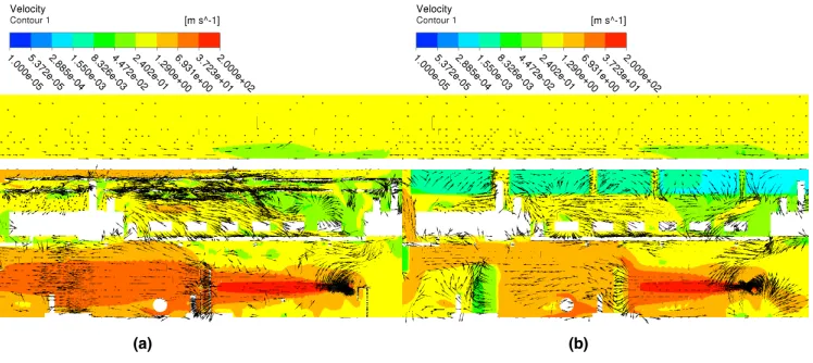
Fig. 3: Contour plots of velocity magnitude: (a) mesh with resolved small-scale objects and (b) mesh with small-scale objects represented using porous regions.

shown on this figure to indicate the flow pattern. These figures show that large-scale flow features are similar for the two geometries. However, one can see differences in the porous regions in terms of both the flow pattern and the velocity magnitude. In the resolved geometry, the flow is predominantly uniform in the region with small-scale piping, whereas when porous regions are used there is some flow re-circulation within the porous regions and the flow velocity is low in these porous regions. In addition, in the resolved geometry a small structure is present roughly 3 meters downstream of the leak. In the porous geometry this structure is represented using a porous box. Figure 3(b) shows that this porous box slows down the flow significantly.

Fig. 4: Vertical velocity profiles downstream of the leak for the two geometry representa-tions.

Fig. 4 shows the velocity profiles along the vertical axis, 9 m downstream of the leak. This figure further shows that the velocity values are higher for the resolved geometry, indicating that there is a momentum loss in the porous domain due to the presence of a porous box.

4.2. Comparison with experimental data

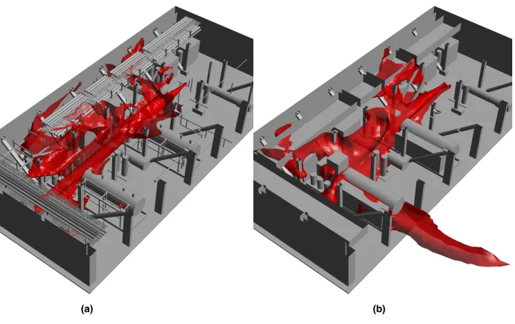
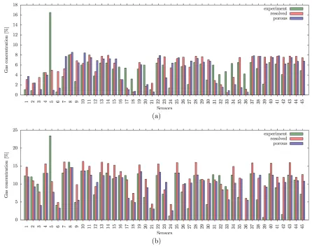
Figure 6(a) and Figure 6(b) respectively show comparison of natural gas concentrations for the experiments, resolved geometry and geometry with porous regions for the two test cases. Following the observation made my Hansen et al. [14] the gas sensors 46-50, which are moved around inside the module for each test case and located inside the jet plume cannot be trusted and is therefore not used in the post-processing. It can be seen that the numerical results predict the same general trend as the measurements, except for sensor 5, which is just downstream of the actual leak.

(a)

(b)

The results from these simulations show that for majority of the sensor for both test 16 and 17, the differences in concentrations between resolved and porous methods is below 50%. The percentage differences are only large for sensors that recorded a low value. However, there were significant differences between both numerical results and the measured data.

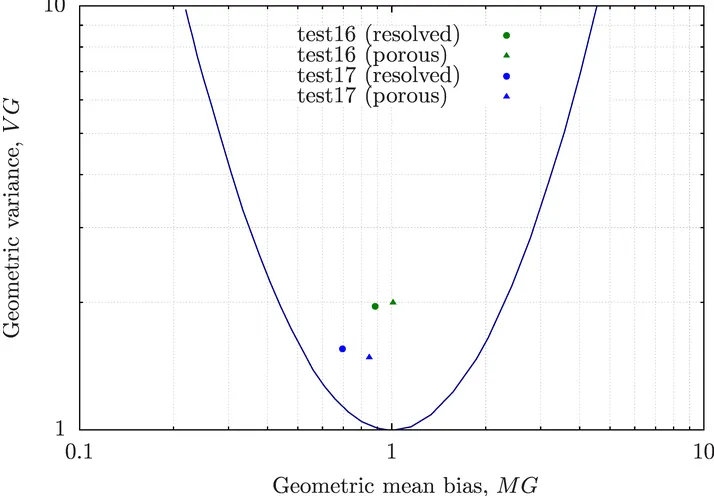
A popular statistical method to compare gas dispersion simulations is to determine the geometric mean and variance for the results, which is shown in Figure 7. A geometric mean and variance of 1 indicates perfect agree-ment. According to this figure there are significant differences between the measurements and numerical results.

Fig. 7: Geometric mean and variance showing the performance of the 4 simulations with experimental measurements.

varied between 110◦ to 210◦. Therefore, the assumption of steady-state wind boundary conditions used in this numerical work is questionable and one may have to include transient boundary conditions to accurately predict the wind profile. In addition, the wind speed was only measured at 20 m above ground, and there are no available data for heights below this. Therefore, the wind profile used in the numerical simulations may be significantly different from experiments.

5. Conclusions

Representing small-scale obstacles using the porosity method gives sig-nificant savings in computational time, both in terms of mesh generation and flow simulation. The porosity method is able to predict large scale flow features obtained using the resolved geometry and the difference in natural gas concentrations obtained from the majority of monitor points for these two geometries are below 50%.

Therefore, the porosity-based geometry used in this work gives accept-able results when compared with the fully resolved geometry. However, the porosity approach needs to be refined further, which will be the focus of a future study.

The large differences between numerical and experimental results could also be due to the assumption of steady-state wind conditions. Unfortunately in experiments such as the ones considered in this work, the wind direction and speed changes considerably. Ideally, one needs to run a transient simu-lation with transient boundary conditions to account for this.

Acknowledgements

The authors would like to thank Innovate UK and DNV GL for their financial support in carrying out this research.

References

[1] S. V. Patankar, D. B. Spalding, A calculation procedure for the transient and steady-state behavior of shell-and-tube heat exchangers, McGraw-Hill New York, 1974.

[3] C. E. Fothergill, S. Chynoweth, P. Roberts, A. Packwood, J. Loss Pre-vent. Proc. 16 (2003) 341–347.

[4] C. Savvides, V. Tam, D. Kinnear, in: Major hazards offshore, p. 07489.

[5] M. J. Ivings, M. Azhar, C. Carey, C. J. Lea, S. Ledin, Y. Sinai, C. Skin-ner, P. Stephenson, Outstanding safety questions concerning the use of gas turbines for power generation–Final report on the CFD mod-elling programme of work, Health and Safety Laboratory, 2003. Report CM/03/08.

[6] B. H. Hjertager, T. Solberg, K. O. Nymoen, J. Loss Prevent. Proc. 5 (1992) 165–174.

[7] D. M. Johnson, R. P. Cleaver, Gas explosions in offshore modules fol-lowing realistic releases (Phase 3B)–Final summary report, Advantica Technology, 2001.

[8] C. D. Argyropoulos, N. C. Markatos, Appl. Math. Model. 39 (2015) 693–732.

[9] ANSYS, ANSYS CFX-Solver Theory Guide, ANSYS, Inc., 2013.

[10] N. R. Popat, C. A. Catlin, B. J. Arntzen, R. P. Lindstedt, B. H. Hjertager, T. Solberg, O. Saeter, A. C. Van den Berg, J. Hazard. Mater. 45 (1996) 1–25.

[11] R. B. Bird, W. E. Stewart, E. N. Lightfoot, Transport Phenomena, Wiley, New York, second edition, 2002.

[12] P. J. Richards, R. P. Hoxey, J. Wind Eng. Ind. Aerodyn. 46 (1993) 145–153.

[13] B. C. R. Ewan, K. Moodie, Combust. Science Technol. 45 (1986) 275– 288.