Munich Personal RePEc Archive
Institutions and growth: Testing the
spatial effect using weight matrix based
on the institutional distance concept
Ahmad, Mahyudin and Hall, Stephen G.
Universiti Teknologi MARA, University of Leicester
19 July 2012
Online at
https://mpra.ub.uni-muenchen.de/42294/
1
Institutions and Growth: Testing the Spatial Effect
Using Weight Matrix Based on the Institutional
Distance Concept
Stephen G. Hall
Professor of Economics, University of Leicester, LE1 7RH Leicester, United Kingdom and University of Pretoria
Mahyudin Ahmad
Corresponding author. Universiti Teknologi MARA, Kedah, P.O. Box 187, 08400 Merbok, Kedah, Malaysia.
604-4562563 / 6012-5236356
604-4562234
Abstract:
This study augments a standard growth model with institutional controls, and models the spatial dependence using geographical and institutional weight matrices. Spatial Durbin model is shown to be the most appropriate to describe the data and political institutions weight matrix best explains the institutional distance concept since it produces identical results to the exogenous geographical-based distance matrix. Overall, the findings give evidence to the institutional quality effects, particularly the security of property rights, on economic growth in the developing countries. We also find evidence of an indirect route of institutions spillover where institutions in a country lead to economic improvement in that country and generate positive effects on the neighbouring
countries’ income growth. Furthermore, our study is able to show that countries with similar political
institutional settings have an increased spatial dependence and converge to a similar level of growth.
Keywords: Growth, institutions, spillover effects, institutional distance, spatial Durbin model.
2
1. Introduction
This paper contributes to the literature on growth and institutional quality by investigating a
growth model which incorporates spatial effects based both on a conventional distance
measure and a novel approach using a spatial weighting matrix based on institutional
closeness. The intuition behind this paper is that the errors in a panel growth regression
contain, at least in part, all the misspecification and omitted variables in the model.
Institutional quality is hard to measure and so any index of quality must be subject to
problems which will be reflected in the errors of the model. We would therefore expect that
similar countries in an institutional sense will exhibit similar errors. This is the essence of the
spatial institutional model we propose here. This study then examines spatial spillover effect
of institutional quality and attempts to uncover the channel through which the institutional
spatial spillover effect works, and hence explains the convergence process for countries with
similar institutional settings.
A standard growth model is augmented with institutional variables to proxy for property
rights and political institutions to test for the absolute effect of the institutional quality. To
account for institutional spatial dependence, specific controls connecting the countries under
study via various weight matrices are used. In addition to an exogenous weight distance
matrix, this study introduces a new spatial weight matrix based on an institutional distance
concept which has never been formally modelled previously. Two-stage testing is conducted
to determine the most appropriate spatial model to be used.
Overall, this study finds substantial institutional spatial dependence in the countries under
study, and the preferred model is one with spatially lagged dependent and explanatory
variables. Furthermore, the institutional weight matrix based on endogenous political
institutional variables is shown to perform empirically well in explaining the institutional
distance since it produces similar results to that of exogenous geographical-based weight
matrix. The findings of this study give support to significant institutions’ absolute effect on
economic growth in developing countries particularly the property rights institutions.
Institutional spatial spillover is shown to exist between the countries, at least via an indirect
route. In other words, an improvement in the quality of institutions in a country lead to
economic improvement in that country and subsequently impact on the neighbouring
3 institutional settings have an increased spatial dependence and eventually converge to similar
level of growth.
The study is organized as follows: Section 2 presents a brief review of institutional spatial
studies, followed by a discussion of the empirical framework in Section 3 and estimation
strategy and data sources in Section 4. Section 5 explains the estimation results and Section 6
concludes with some remarks on the limitation of this study.
2. Brief review of the institutional spatial literature
The growth literature has investigated the significance of spacial effects on economic growth,
see for instance an excellent survey by Abreu, et al. (2005) on the space-growth relationship,
the empirical evidence and the methods widely used to test the relationship. The main
channels through which space affects regional economic activity can be explained in term of
absolute and relative location effects.
Absolute location effect refers to the impact of being located at a particular point in space, for
instance in a certain region or climate zone, or at a certain latitude, while relative location
effect refers to the impact of being located closer or further away from other specific
countries or regions. The relative effect is related to the concept of spatial dependence, which
according to Anselin and Bera (1998), Anselin (2001) and Arbia (2006), if omitted, leads the
standard growth model to be seriously misspecified. Abreu et al. (2005) note that a cluster of
low growth regions could somehow be the results of spillover from one region to another and
the effects could be emanating from numerous factors such as climate, technology, or
institutions1.
Theoretically, Bosker and Garretsen distinguish three possible channels through which the
institutional setup of country i can have an impact on the income of country j, and they are either indirect or direct, or via an influence on the quality of institutions in country j and thereby on the income in country j. They are defined as follows:
1
As far as the institutional impact on growth is concerned, on overall, it is fair to say that the institutional
4 i. An indirect spatial institutional effect is when institutions in a neighbouring country
lead to economic, social, or political outcomes in that country which in turn have an
impact on the home country’s income level (see Easterly and Levine 1998; Ades and
Chua 1997; Murdoch and Sandler 2002).
ii. The direct route is when institutions in a neighbouring country produce spillover
effect on economic, social, or political outcomes in the home country and thereby
impact the country’s income level (see Gleditsch and Beardsley 2004; Salehyan and
Gleditsch 2006; Salehyan 2008 in the political science literature; and Kaminsky and
Reinhart 2000 in the trade and financial flow literature).
iii. The last channel relates to the concept of institutional spatial spillover where the level
of neighbouring institutions affects the quality of home country’s institutions and
thereby impacting the home countries’ income level (See Kelejian et al. 2008; Faber
and Gerritse 2009).
Empirically, there are a number of studies whose findings support the existence of
institutional spatial dependence between neighbouring countries. For example, Easterly and
Levine (1998) find evidence of spillover effects between growth in African countries and
their neighbours suggesting that the copying of policies might be partially responsible for this
relationship2. Simmons and Elkins (2004) examine the determinant of changes in policy
regimes and find that switches between regimes can be explained by policy choices in
countries experiencing the similar situations. These studies, however, are not based on formal
spatial econometric models.
In a more formal study using an explicit spatial framework, Kelejian et al. (2008) find quality
of institutions in neighbouring countries has a quantitatively important impact on the
institutional development in the home country and this finding is statistically significant and
robust to different empirical specifications3. In spite of similar finding as far as institutional
2
Though the study by Easterly and Levine (1998) does not make an explicit use of spatial econometric model, their estimation method is however consistent with it as they instrument the spatial lag with explanatory variables of the neighbouring countries.
3
5 development in the home country is concerned, Faber and Gerritse (2009) however find no
direct impact of nearby countries’ institutional quality on home country’s income. Similarly
Claeys and Manca (2010) examine the spatial links of different political institutions across
borders by applying various tests for spatial proximity and they find no evidence of
contemporaneous spatial links and they argue this finding is robust to various measures of
distance and of cultural proximity across countries4.
The latter two studies are however in contrast with Ades and Chua (1997) and Murdoch and
Sandler (2002) who find political instability and poor situations (like number of revolutions
and coups, and civil wars) in neighbouring countries negatively affect the economic
performance in the home countries. More recent and formal spatial studies from Bosker and
Garretsen (2009) and Arbia et al. (2010) are able to present strong evidence in favour of the
proposition that institutional quality in neighbouring countries undoubtedly matters for a
country’s economic development.
Arbia et al. empirically investigate the growth experience in European regions during the
period 1991-2004 and models the spatial interdependence using institutional5 and
geographical6 weight matrices. They are able to show that spatial externalities are a
substantive phenomenon7, and find the relative location effect of institutions is highly
significant to regional output per worker. They also find evidence that, holding the
geographical distance fixed, the regions sharing similar institutional characteristics tend to
converge more rapidly to each other.
explanatory variables whose significant impact on institutional development previously documented in the literature are used, such as legal origins, ethnic fractionalisation, religion, natural resources as well as geographical variables. The results are consistent even when different weight matrices used such as common border, length of common border, and inverse distance.
4
Claeys and Manca (2010) use Worldwide Governance Index institutional indicators obtained from the World Bank and Economic Freedom index by Fraser Institute with various weight matrices including geographical measures (contiguity, physical distance), economic linkage (trade, countries stage of development) or ease of exchange across cultures (using measures like linguistic diversity, ethnic and religious fractionalisation, legal origin).
5
Arguably Arbia et al. (2010) are the first to employ institutional weight matrix in spatial study, but they instrument the endogenous institutional matrix using exogenous linguistic distance. Linguistic distance is normally used to reflect obstacles to trade, therefore they inverse linguistic distance to create a measure of language similarity which in turn reflects similar institutional arrangement.
6
In spatial literature, the exogenous geographical-based measures of distance are widely used to establish the linkage via which the spatial dependence between regions/countries runs. Example of the geographical weight matrix will be discussed in empirical framework section.
7
6
3. Empirical framework
Consider a simple growth model based on Barro (1991) as follows:
y X
gt log 0 (1)
where gt logytwhich is an Nx1 vector of real GDP per capita growth rates,
is an Nx1vector of constant terms, logy0is an Nx1 vector of logs of real GDP per capita at the beginning of the period, Xis an Nxk matrix of explanatory variables, is the convergence
coefficient, is Kx1 vector of parameters, and
~ N(0,
2I)is an Nx1 vector of i.i.d. error terms. is the convergence parameter of the countries under study and it is expected to benegative as it shows the catching-up process by the countries to their steady state. A set of
explanatory variables X is added as steady state determinants and following Mankiw et al. (1992) stock of physical (sk) and human (sh) capitals, as well as a term (n+g+δ) that
accounts for the sum of population growth, growth in exogenous technological process, and
depreciation rate, respectively are included. To capture the absolute location effect of
institutions, we augment the model with indices of institutional quality namely the security of
property right index (iiqicrg) and the political institutions index (iiqpol). In full, the matrix of
K explanatory variables is therefore given by X=[sk, sh,n+g+δ, iiqicrg, iiqpol] where each element is an Nx1 vector.
To account for the spatial dependence in the growth model of Equation (1), a spatial
autoregressive error term is considered:
u
W
(2)
where W is an NxN spatial weight matrix incorporating the spatial connections of the system,
λ is a spatial autoregressive parameter, ε is an Nx1 vector spatially correlated errors, and u is an Nx1 vector of a spatial disturbance term with i.i.d. properties.
Assuming the inverse
I W
1exists, and combining Equation (2) with Equation (1), areduced form can be written as:
I W
u Xy
7 where I is the Nx1 identity matrix. However, Equation (3) can be seen as a spatial error model (SEM) growth process where the spatial dependence operates via shocks to the income
growth in the regions. The term
IW
1can be decomposed into:
1(
) 2 2 ...
W W I W W
I
o i
i
i
(4)
From this decomposition, the spatial autocorrelation is therefore assumed to be a global
process as the country-specific shocks propagate themselves to neighbouring countries via a
weight matrix. Notwithstanding that, this decomposition also renders the spatial externalities
a nuisance factor since it operates through the “error term” which rather makes the spatial
effect a relatively less important in the model (Arbia et al. 2010).
However Equation (4) above can be rearranged to model a more direct or more substantive
effect of the spatial relationship, which is the following:
u WX y
W Wg X
y
g
log 0
log 0
(5)where
is vector of constants i.e. (1W), and and . It transforms into the Spatial Durbin Model (SDM) which incorporates a spatially lagged dependent variableand spatially lagged explanatory variables. and will be the restrictions for
Equation (5) and these restrictions enable us to test whether spatial dependence is a nuisance
factor that runs via error structure or a substantive factor which directly impacts the growth
via endogenous (spatially lagged dependent variable) and exogenous variables (spatially
lagged explanatory variables) of the model. We will discuss the test for these restrictions
more in the next section.
Thus, if the convergence speed in the normal growth equation is given by the convergence
coefficient, which is the partial derivative of the per capita income growth with respect to
the initial income per capita, a model with spatially augmented growth and initial income will
thus transforms the convergence coefficient into an augmented partial derivative.
Specifically, a closer look at the spatial Durbin model in Equation (5) reveals that it can be
8 )
log log
( ) 1
( W 1 y0 X W y0 WX u
g
(6)and therefore, the partial derivative of the per capita income growth with respect to the initial
income per capita is given by:
) (
) 1 ( log
/ y0 W 1 I W
g
(7)
Since the spatial weight matrix is row standardized, and assuming, after the expansion in
Equation (4), the effect of higher orders spatial terms rapidly approach zero and rounding it to
first order effect only, the augmented convergence coefficient is therefore:
) 1
( (8)
which makes the convergence speed now influenced by the neighbouring effects. In other
words, the speed of convergence in the spatial model can be shown to be higher than the
normal beta convergence due to the spatial spillover effects8.
As introduced in the Equation (2) above, W is the NxN spatial weight matrix that becomes the linkage among the countries in the sample. It is usually specified via a number of
geographical measures of distance such as physical distance, contiguity measures, k-nearest regions, or a more complex decay function. The advantage of using geographical-based
distance is that it is unambiguously exogenous to the model, and therefore it eliminates the
problem of identification and causal reversion. However in this study, in addition to a
geographical-based weight matrix, we go on to also use a weight matrix based on institutional
similarity which is a novel extension to the standard model.
In this study, we use row standardized inverse squared distance9 (denoted winvsq) whose elements are defined according to a gravity function that provides an exponential distance
decay. Thus, the spatial relationship using this weight matrix is modelled according to the
concept of impedance, or distance decay. All features influence all other features, but the
8
We follow Arbia et al. (2010) to assume so to make the augmented convergence speed easier to compute. 9
We use latitude and longitude data to compute the Great Circle distance i.e. the shortest distance between any two points on the surface of a sphere measured along a path on the surface of the sphere (as opposed to going through the sphere's interior). It is computed using the equation:
sin sin cos cos cos
arccos i j i j
ij
d
where iand jare the latitude of country i and j respectively, and denotes the absolute value of the
9 farther away something is, the smaller the impact it has. Because every feature is a neighbour
of every other feature, a cut-off distance needs to be specified to reduce the number of
required computations with large datasets, and we set it at minimum threshold which will
guarantee that each countries has at least one neighbour. The matrix W is given by:
0
ij
w
if i j
j ij ij
ij d d
w 2 2
if 2 2 d dij 0 ij w if otherwise ( 9)
where dijis the great circle distance between country capital i and j, and dis the critical distance cut-off after which spatial effect is considered to be negligible. The elements of the
main diagonal are set equal to zero by convention since a country cannot be a neighbour to
itself. Since the data used in this study consists of i=1 to n=58 countries, and similarly the
corresponding countries’ capitals to calculate the distance is j=1 to k=58, and the time period
is t=1984 to T=2007, the distance weight matrix for a particular year, t, will be:
0 0 0 , , , , , , in t jn t jk t ji t ik t ij t t w w w w w w
W ( 10)
and stacking the matrix first by time and then by cross section gives the full weighting matrix
as: T t t W W W W 0 0 0 0 0 0 2 ( 11)
with a dimension of 58*24x58*24 i.e. 1392x1392.
Arbia et al. (2010) include a non-conventional weight matrix based on institutional
heterogeneity between institutions in addition to geographical-based ones. They argue this
new matrix can capture distance which is not geographically based yet still play an important
10 role in shaping the economic behaviour both at micro and macro level. In this study, we
formally integrate the institutional distance10 into the spatial estimation by using a weight
matrix constructed based on Kogut and Singh (1988) cultural distance (CD) index calculation
as in Equation (12) below:
n
V I I CD
n
i
i ik ij
1
2
/ ) (
( 12)
where Iijis the index value for cultural dimension i for country j,Iikis the index value for
cultural dimension i for country k, Viis the variance of the index of the cultural dimension i, and
n
is the number of cultural dimension i. In our study, we replace the cultural dimension with institutional dimensions constructed from four institutional indicators (therefore fourdimensions) from the International Country Risk Guide (ICRG) database to construct an
index to reflect the security of property rights (denoted wicrg), and four political institutions indicators from four different sources to construct an index of political institutions (denoted
wpol). These institutional distance matrices are computed for each year for the whole sample period of 24 years and then stacked to complete the weighting matrix as in Equation (11).
We fully acknowledge that there is a possibility of an endogeneity issue in the use of these
institutional matrices11. Notwithstanding that, the primary motivation of this study is to gauge
the effect of institutional proximity to economic growth and therefore these matrices are of
primary interest, and to mitigate this endogeneity issue, an exogenous weight matrix based on
geographical distance is used as a benchmark against which the results of the estimation
using institutional-based weight matrices are interpreted.
4. Estimation strategy and data sources
The dataset used in this study consists of a panel observation for 58 developing countries in
three regions namely Africa, East Asia, and Latin America for a period of 24 years beginning
10
Institutional distance concept is actually widely researched in the field of international management and international business based on the works by Kostova (1999) and Kostova and Zaheer (1999). They build on the
Scott (1995)’s framework outlining three pillars of institutionalism to define institutional distance as the extent to which regulative, cognitive and normative institutions of two countries differ from one another. We are however more interested in the way the institutional distance is measured in the international management literature using Kogut and Singh index of cultural distance.
11
11 from 1984 to 2007. Data on real GDP per capita and population growth are obtained from
World Development Indicators (WDI) from the World Bank (2009). We follow Mankiw et
al. (1992), Islam (1995), Caselli et al. (1996) and Hoeffler (2002) to assume exogenous
technological change plus depreciation rate (g+δ) as 0.05. We also follow them to use
investment share of real per capita GDP as a proxy for capital and the investment data is
obtained from Penn World Table 6.3 (Heston et al. 2009). To proxy for human capital, we
use secondary school attainment for population age 15 and above from Barro and Lee (2010)
educational data12. To measure formal institutional quality parameters that reflect security of
property rights and the political institutions, we utilize institutional indicators from five
sources. They are (1) International Country Risk Guide (ICRG) obtained from the PRS Group
(2009) from which we use four variables –Investment Profile, Law and Order, Bureaucracy
Quality, and Government Stability, (2) Polity IV data (Marshall and Jaggers 2008) –Polity2
variable, (3) Freedom in the World index also known as Gastil index (Gastil 1978) –Political
rights variable, (4) The Political Constraint Index (POLCON) Dataset (Henisz 2010) –
Polcon3 index, and (5) Database of Political Institutions by the World Bank (Beck et al.,
2001) –Checks variable. To estimate the absolute location effect of institutions, we use
simple average of the four ICRG indicators to make up the first index of institutional quality
(iiqicrg) and this index reflect security of property right dimension, whereas simple average of the four political indicators from four different sources become the second index of
institutional quality (iiqpol) and this index reflect the political institutions.
To estimate the growth model, four different specifications are employed, all with real GDP
per capita growth (g) as the dependent variable, and log of initial income (log y1984) as the
variable to test for the convergence effect. Model (1) is a baseline model with only Mankiew,
Romer and Weil (1992) –henceforth MRW– variables i.e. physical (sk) and human capitals (sh) and a sum of population growth, exogenous technological process and depreciation rate (n+g+δ). Model (2) and (3) introduce institutional controls using iiqicrg and iiqpol indices, respectively, and finally Model (4) is the general model where both institutional indices enter
the equation simultaneously.
The empirical analysis begins with testing for the spatial autocorrelation in the model.
Equation (1) is estimated via Ordinary Least Square (OLS) and the presence of spatial
12
12
autocorrelation in the residuals is tested using Moran’s I test. If the presence of spatial
autocorrelation is detected, OLS is then rejected because its estimates are no longer
appropriate for models containing spatial effects. In the case of spatial autocorrelation in the
error term, the OLS estimates of the response parameter remains unbiased, but it loses its
efficiency property, and in the case of specification containing spatially lagged dependent
variable, the estimates are not only biased, but also inconsistent13. It is therefore commonly
suggested that maximum likelihood regression technique should be used to overcome this
problem (see Elhorst 2003).
Having detected the presence of spatial effects we then proceed to determine the appropriate
form of spatial model to use. LeSage and Pace (2009) argue that the spatial Durbin model is
the best point to begin the test since the cost of omitting the spatially autocorrelated error
term is less (efficiency loss of the estimators) compared to the cost of ignoring the spatially
lagged dependent and independent variables (the estimators are biased and inconsistent).
However, Florax et al. (2003) argue that using spatial lag model, conditional on the results of
misspecification tests, outperforms the general-to-specific approach for finding the true data
generating process14.
In this study, two-stage testing process is used to determine the model that best fits the data.
In the first stage, we use the robust Lagrange Multiplier (LM) tests developed by Anselin et
al. (1996) to decide which model between the spatial error model and the spatial lag model
that is better-suited to the data. It is called robust because the existence of one more type of
spatial dependence does not bias the test for the other type of spatial dependence. This
characteristic is obviously important because we will omit the spatial model that fails this test
in most cases when estimated with different model specifications and using different weight
matrices. The model that succeed in the first stage test will then be tested against the general
model i.e. the spatial Durbin model in the second stage using the Likelihood ratio (LR) test
for the spatial common factors. The LR test is as the following:
) ( ~ ) (
2 L L 2 k
LR ur r
(13)
13
Notwithstanding that, inconsistency is only a minimal requirement for a useful estimator. 14
13 Due to Elhorst (2010) which is partly based on Elhorst and Fréret (2009), and Seldadyo et al.
(2010). To carry out the second stage testing, we estimate spatial Durbin model as the
unrestricted model, and test it against the restricted model which is either the spatial lag or
error model that succeeds in the first stage test.
5. Estimation results and discussions
Table 1 presents the results of standard OLS regression of the four growth models in
Equation (1). These all fit the stylized facts about the presence of conditional convergence in
developing countries. The coefficients for initial income are consistently negative and
statistically significantly different from zero. Coefficients of the other growth determinants
are also statistically significant with the expected sign except population growth which is
positive. It is however not surprising to have positive population growth effect on economic
growth especially in developing countries as shown by Headey and Hodge (2009) who found
[image:14.595.89.511.412.755.2]no strong support for the opposite hypothesis.
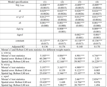
Table 1: Standard OLS growth regression and Moran's I test for spatial autocorrelation in residualsa Model specification (1) (2) (3) (4)
log y1984 -0.008*** -0.009*** -0.009*** -0.009***
(0.0015) (0.0015) (0.0015) (0.0016) sk 0.029*** 0.025*** 0.028*** 0.024***
(0.0026) (0.0026) (0.0026) (0.0027) n+g+δ 0.012*** 0.011*** 0.012*** 0.011***
(0.0016) (0.0016) (0.0016) (0.0016) sh 0.001*** 0.001*** 0.001*** 0.001***
(0.000) (0.000) (0.001) (0.000)
iiqicrg 0.008*** 0.009***
(0.001) (0.001)
iiqpol 0.002*** 0.001*
(0.001) (0.001) constant -0.115*** -0.126*** -0.118*** -0.136***
(0.017) (0.017) (0.017) (0.017) Adjusted R2 0.136 0.176 0.140 0.170
Moran’s I and Robust LM tests statistics for different weight matrix: a. winvsq
Moran’s I test statistics 5.185*** 4.884*** 4.901*** 4.744*** Spatial error: Robust LM test 40.286*** 1.768 34.930*** 2.53 Spatial lag: Robust LM test 67.543*** 12.168*** 59.907*** 14.229*** b. wicrg
Moran’s I test statistics 5.197*** 3.163*** 4.989*** 3.316*** Spatial error: Robust LM test 10.533*** 0.339 9.123*** 0.005 Spatial lag: Robust LM test 25.030*** 2.346*** 23.107*** 0.788 c. wpol
Moran’s I test statistics 2.735*** 2.690*** 2.667*** 2.854*** Spatial error: Robust LM test 19.620*** 1.448 14.704*** 0.076 Spatial lag: Robust LM test 28.111*** 5.082** 20.793*** 1.494 a
14
only MRW variables i.e. sh, sk, and n+g+δ, model (2) with MRW variables and iiqicrg, (3) with MRW variables and iiqpol, and (4) with MRW variables, and both iiqicrg and iiqpol indices. Standard errors are in parentheses. ***, ** and * denote significance at 1%, 5% and 10% respectively.
The result of Moran’s I test in Table 1 indicates that the null hypothesis of no global spatial
autocorrelation in the residuals of the OLS regression is overwhelmingly rejected. This
finding holds when different weight matrices are used including the geographical- and
institutional-based. Hence, it can be safely inferred that Equation (1) is misspecified and the
OLS estimates are invalid. The model therefore should be modified to include spatial
dependence term. From the robust LM test statistics, the spatial error model is apparently
inappropriate as it fails in a number of cases (specifically in model (2) and (4)) compared to
spatial lag model. The LR tests statistics for the common factors between spatial lag and
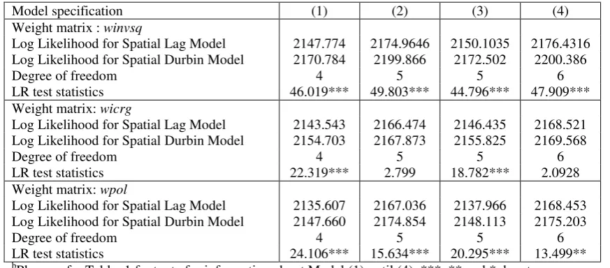
spatial Durbin model are used to decide which of the two models best explains the data.
Based on the result in Table 2 it is particularly obvious that spatial Durbin model is favoured
[image:15.595.81.518.409.601.2]over the spatial lag model.
Table 2: Likelihood ratio test between spatial Durbin and spatial lag modelb
Model specification (1) (2) (3) (4) Weight matrix : winvsq
Log Likelihood for Spatial Lag Model 2147.774 2174.9646 2150.1035 2176.4316 Log Likelihood for Spatial Durbin Model 2170.784 2199.866 2172.502 2200.386
Degree of freedom 4 5 5 6
LR test statistics 46.019*** 49.803*** 44.796*** 47.909*** Weight matrix: wicrg
Log Likelihood for Spatial Lag Model 2143.543 2166.474 2146.435 2168.521 Log Likelihood for Spatial Durbin Model 2154.703 2167.873 2155.825 2169.568
Degree of freedom 4 5 5 6
LR test statistics 22.319*** 2.799 18.782*** 2.0928 Weight matrix: wpol
Log Likelihood for Spatial Lag Model 2135.607 2167.036 2137.966 2168.453 Log Likelihood for Spatial Durbin Model 2147.660 2174.854 2148.113 2175.203
Degree of freedom 4 5 5 6
LR test statistics 24.106*** 15.634*** 20.295*** 13.499** b
Please refer Table 1 footnote for information about Model (1) until (4). ***, ** and * denote significance at 1%, 5% and 10% respectively.
Now we turn to the estimation of Spatial Durbin model as in Equation (5) with three different
weight matrices i.e. inverse squared distance (winvsq), the security of property rights index (wicrg) and the political institutions index (wpol) and the results of these models are presented in the Tables 3, 4 and 5, respectively.
15 Overall, the results support the conditional convergence hypothesis. The coefficients of initial
income are always negative and significant across all estimations, The coefficients of the
steady state determinants i.e. physical and human capitals are also positive and significant.
The positive effect of population growth towards economic growth also remains.
The absolute effect of institutional quality on growth mirrors the result in the standard OLS
growth regression especially in the models containing the iiqicrg index as it is always significant, whereas in most cases, the iiqpol index is not. The iiqicrg index however seems to be sensitive to the choice of the weight matrix as it only becomes significant when winvsq
and wpol are used, and not when wicrg is used.
The coefficients for the spatially lagged dependent variables, , are positive and significant
across all model specifications using the three weight matrices at least at 10% level and the
Wald test for the null hypothesis of 0 are overwhelmingly rejected. This finding gives
convincing support to the proposition of positive spatial autocorrelation in per capita income
growth of the developing countries. Since positive absolute effect of institutional quality
towards per capita income growth is reported in the preceding paragraph, this further
confirms the existence of the institutional spatial dependence between the countries, at least
via the indirect route, where institutions in a country lead to economic improvement in that
country (absolute effect) and generate spillover effect to neighbouring countries’ income
growth (relative effect).
This finding is apparently similar to Easterly and Levine (1998), Ades and Chua (1997),
Murdoch and Sandler (2002), Bosker and Garretsen (2009) and Arbia et al. (2010) who find
evidence of positive spillover effect of growth in neighbouring countries to home countries’
growth. The Wald test for the null hypothesis that the coefficients of the spatially lagged
explanatory variables are equal to zero is also rejected in almost all cases (except (2) and (4)
when wicrg is used) and this is a clear indication that the spatial Durbin model is the most appropriate to explain the data.
The coefficients of spatially lagged initial income, though they are not significant in most
16 lagged initial income is that the relative location of the developing countries, due to their
proximity in physical space and institutional settings, generates spillover effect that operates
only via the spatial per capita income growth process, and not via the spatially lagged initial
income. This situation could points to a possibility that the developing countries under study
do not essentially share similar long run growth determinants which otherwise would have
caused an influence to spatial conditional convergence and allowed the countries to converge
to the same long run growth path (see Abreu et al. 2005 and Arbia et al. 2010 for more
discussion on spatial conditional convergence process).
For the augmented convergence speed, it is apparently higher than those obtained from the
standard growth regressions once the magnitude of the neighbourhood effect is accounted.
The rate of speed rises from 0.8-0.9% in standard growth regression (Table 1) to 1.9-2.2% in
spatial growth regression with winvsq matrix (Table 3). This finding therefore confirms the
positive effect of neighbouring countries’ per capita income growth on home countries per
capita income growth and suggests countries that belong to the same clusters in space tend to
converge to a similar level of growth.
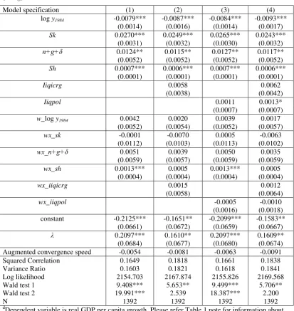
As for the model with institutional distance matrices, the regression using wpol matrix gives identical results to the model using winvsq matrix with convergence speed greater than that of standard regression and this gives an indication that countries with similar level of political
institutional settings tend to converge to similar level of growth. However, in regression
using the wicrg weight matrix, the augmented speed of convergence however is much lower than that of standard growth regressions and we are of the opinion that the reason to this
finding is because of the weakness of wicrg as a weight matrix.
The estimation results also yield positive significant spatial externalities of the physical and
human capitals (wx_sk and wx_sh respectively) i.e. there is significant spatial dependence in the physical and human capitals among the countries. This is not uncommon in the
growth-space literature as shown by Lall and Yilmaz (2001) who estimate a conditional convergence
model with human capital spill overs using data for the United States and they find evidence
that human capital levels are spatially correlated. López-Bazo et al. (2004) meanwhile find
evidence of technology diffusion in the EU regions where the level of technology in each
17 physical and human capitals. Ertur and Koch (2006; 2007) propose a spatially augmented
Solow model that is able to show the technological interdependence, and spatial externalities
of physical (2007) and human capitals (2006). Again, estimation using wicrg matrix produce insignificant spatially lagged physical and human capitals in most cases.
Similar to its absolute effect, the relative effect of the institutional index, particularly iiqicrg, remains significant in all models estimated with matrix winvsq and wpol, but not with wicrg. On the other hand, the relative effect of iiqpol index is found to be insignificant most of the time. Contrary to the previously documented positive spillover effect of institutions towards
growth (as earlier discussed in the review section, and see also Easterly and Levine 1998;
Ades and Chua 1997; Murdoch and Sandler 2002; Bosker and Garretsen 2009; and Arbia et
al. 2010), we however find negative spillover effects of the iiqicrg index. In hindsight, these contradictory findings could be thought of as the consequence of an endogeneity problem that
plagues the spatial model estimation using institutional weight matrix (wicrg and wpol). Nevertheless, the relative effect of iiqicrg remains negative in the estimation using the
exogenous geographical-based matrix (winvsq). This study is not the first to find no empirical support for the positive spillover effect of institutions since Faber and Gerritse (2009) and
18
Table 3: Spatial Durbin regression of growth model using inverse squared distance weight matrix (winvsq)c
Model specification (1) (2) (3) (4) log y1984 -0.0058*** -0.010*** -0.0059*** -0.0099***
(0.0014) (0.0018) (0.0015) (0.0018) sk 0.0184*** 0.0137*** 0.0179*** 0.0135***
(0.0029) (0.0030) (0.0029) (0.0031) n+g+δ 0.0146*** 0.0138** 0.0147*** 0.0138** (0.0055) (0.0054) (0.0055) (0.0054) sh 0.0008*** 0.0006*** 0.0007*** 0.0006***
(0.0001) (0.0001) (0.0001) (0.0001) iiqicrg 0.0093*** 0.0091***
(0.0021) (0.0021)
iiqpol 0.0010 0.0005
(0.0007) (0.0006) w_ log y1984 -0.0150*** -0.0080 -0.0143*** -0.0073
(0.0051) (0.0056) (0.0051) (0.0057) wx_sk 0.0408*** 0.0429*** 0.0442*** 0.0445***
(0.0087) (0.0089) (0.0091) (0.0090)
wx_n+g+δ 0.0056 0.0035 0.0031 0.0020
(0.0088) (0.0087) (0.0089) (0.0090) wx_sh 0.0013*** 0.0016** 0.0014*** 0.0016***
(0.0005) (0.0006) (0.0005) (0.0006) wx_iiqicrg -0.0123*** -0.0118***
(0.0041) (0.0042)
wx_iiqpol -0.0040* -0.0023
(0.0024) (0.0025) constant -0.1978* -0.1805* -0.1821* -0.1737* (0.1092) (0.1018) (0.1090) (0.1025) λ 0.1749** 0.2038*** 0.1802** 0.2057***
(0.0705) (0.0700) (0.0701) (0.0699) Augmented convergence speed -0.0218 -0.0200 -0.0213 -0.0192 Squared Correlation 0.1844 0.2164 0.1864 0.2169 Variance Ratio 0.1849 0.2160 0.1862 0.2164 Log likelihood 2170.784 2199.866 2172.502 2200.386 Wald test 1 6.160** 8.476*** 6.606*** 8.665*** Wald test 2 31.386*** 30.522*** 34.904*** 32.253***
N 1392 1392 1392 1392
c
Dependent variable is real GDP per capita growth. Please refer Table 1 footnote for information about Model (1) until (4). Standard errors are in parentheses. Wald test 1 is for null hypothesis that
λ=0 ~χ 2(1). Wald test 2 is for null hypothesis that coefficients on lags of X's (or spatially lagged
19
Table 4: Spatial Durbin regression of growth model using institutional distance weight matrix (wicrg)d
Model specification (1) (2) (3) (4) log y1984 -0.0079*** -0.0087*** -0.0084*** -0.0093***
(0.0014) (0.0016) (0.0014) (0.0017) Sk 0.0270*** 0.0249*** 0.0265*** 0.0243***
(0.0031) (0.0032) (0.0030) (0.0032) n+g+δ 0.0124** 0.0115** 0.0127** 0.0117**
(0.0052) (0.0052) (0.0052) (0.0052) Sh 0.0007*** 0.0006*** 0.0007*** 0.0006***
(0.0001) (0.0001) (0.0001) (0.0001)
Iiqicrg 0.0058 0.0062
(0.0038) (0.0042)
Iiqpol 0.0011 0.0013*
(0.0007) (0.0007) w_log y1984 0.0042 0.0020 0.0039 0.0017
(0.0052) (0.0054) (0.0052) (0.0057) wx_sk -0.0001 -0.0070 0.0005 -0.0063 (0.0112) (0.0103) (0.0113) (0.0102)
wx_n+g+δ 0.0051 0.0039 0.0050 0.0035
(0.0059) (0.0057) (0.0059) (0.0059) wx_sh 0.0013*** 0.0005 0.0013*** 0.0005
(0.0004) (0.0004) (0.0004) (0.0004)
wx_iiqicrg 0.0015 0.0012
(0.0058) (0.0064)
wx_iiqpol -0.0005 -0.0010
(0.0016) (0.0018) constant -0.2125*** -0.1651** -0.2099*** -0.1583**
(0.0661) (0.0672) (0.0659) (0.0667) λ 0.2097*** 0.1610** 0.2097*** 0.1609**
(0.0684) (0.0677) (0.0680) (0.0674) Augmented convergence speed -0.0054 -0.0081 -0.0063 -0.0091 Squared Correlation 0.1649 0.1818 0.1661 0.1838 Variance Ratio 0.1603 0.1821 0.1618 0.1841 Log likelihood 2154.703 2167.874 2155.826 2169.568 Wald test 1 9.408*** 5.653** 9.499*** 5.706** Wald test 2 19.991*** 2.539 18.387*** 2.200
N 1392 1392 1392 1392
d
Dependent variable is real GDP per capita growth. Please refer Table 1 note for information about
Model (1) until (4). Standard errors are in parentheses. Wald test 1 is for null hypothesis that λ=0 ~χ2(1). Wald test 2 is for null hypothesis that coefficients on lags of X's (or spatially lagged
20
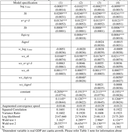
Table 5: Spatial Durbin regression of growth model using institutional distance weight matrix (wpol)e Model specification (1) (2) (3) (4)
log y1984 -0.0085*** -0.0102*** -0.0082*** -0.0099***
(0.0014) (0.0015) (0.0014) (0.0015) Sk 0.0289*** 0.0240*** 0.0290*** 0.0241***
(0.0031) (0.0031) (0.0031) (0.0031) n+g+δ 0.0134*** 0.0122** 0.0133** 0.0121** (0.0052) (0.0052) (0.0052) (0.0051) Sh 0.0008*** 0.0006*** 0.0008*** 0.0006***
(0.0001) (0.0001) (0.0001) (0.0001) Iiqicrg 0.0084*** 0.0084***
(0.0018) (0.0018)
Iiqpol -0.0024 -0.0015
(0.0030) (0.0031) w_log y1984 -0.0051 -0.0020 -0.0038 -0.0009
(0.0036) (0.0036) (0.0039) (0.0038) wx_sk 0.0160** 0.0190*** 0.0176** 0.0211***
(0.0074) (0.0072) (0.0077) (0.0074)
wx_n+g+δ 0.0063 0.0046 0.0055 0.0036
(0.0061) (0.0058) (0.0062) (0.0059) wx_sh 0.0011*** 0.0007** 0.0011*** 0.0007** (0.0003) (0.0003) (0.0003) (0.0003) wx_iiqicrg -0.0048* -0.0050* (0.0028) (0.0027)
wx_iiqpol 0.0021 0.0008
(0.0035) (0.0036) constant -0.2050*** -0.1915** -0.2115*** -0.1951**
(0.0774) (0.0825) (0.0778) (0.0826) λ 0.1145* 0.1287** 0.1111* 0.1268** (0.0644) (0.0622) (0.0645) (0.0624) Augmented convergence speed -0.0146 -0.0135 -0.0129 -0.0121 Squared Correlation 0.1601 0.1916 0.1608 0.1922 Variance Ratio 0.1602 0.1920 0.1608 0.1923 Log likelihood 2147.660 2174.854 2148.113 2175.203 Wald test 1 3.162* 4.289** 2.966* 4.124** Wald test 2 20.557*** 16.654*** 20.130*** 16.581**
N 1392 1392 1392 1392
e
Dependent variable is real GDP per capita growth. Please refer Table 1 note for information about
Model (1) until (4). Standard errors are in parentheses. Wald test 1 is for null hypothesis that λ=0 ~χ2(1). Wald test 2 is for null hypothesis that coefficients on lags of X's (or spatially lagged
explanatory variables)=0 ~χ2(1). ***, ** and * denote significance at 1%, 5% and 10% respectively.
6. Concluding remarks
This study empirically supports the existing evidence on the positive significant absolute
effect of institutions towards economic growth in developing countries. It also finds that
institutional spatial dependence in the countries under study does exist, and institutional
spillover effects are shown to run via the indirect route i.e. institutions in a country lead to
improvement in economic growth in that country and this situation consequently generates
21 of Easterly and Levine (1998), Ades and Chua (1997), Murdoch and Sandler (2002), Bosker
and Garretsen (2009), and Arbia et al. (2010).
However, the spillover effect is found to operate only via spatially lagged per capita income
growth, but not via spatially lagged initial income. This could possibly be due to the fact that
developing countries under study do not share similar long run growth determinants hence
the spatial divergence process. Furthermore, this study is also unable to find conclusive
evidence on the direct channel of the effect for institutional spatial spillover since spatially
lagged institutional variables have on overall negative coefficient (which is against the
convention) and, in most cases, insignificant. This finding therefore effectively confirms the
previously reported indirect channel of institution spillover effects.
With regard to the best institutional weight matrix to proxy for institutional proximity
between the countries, the spatial matrix based on political institutional variables dominates
that of security of property rights since the estimation using the former produces identical
results to the estimation using an exogenous geographical-based matrix. This finding also
implies that countries with a similar level of political institutional settings tend to converge to
similar level of growth. This study also shows the presence of spatial externalities in human
and physical capitals which are also in line with the findings in the previous literature.
Several limitations still abound. Endogeneity remains an important issue and it is not properly
addressed in this study. The use of institutional weight matrix also suffers problem of
endogeneity and one possible remedy to this problem is via instrumenting the matrix with an
appropriate proxy, such as linguistic distance (see Arbia et al, 2010). Notwithstanding that,
considering this is one of the rare attempts to formally model institutional spatial
interdependence via an institutional distance matrix, and arguably the first to focus on
developing coutnries15.
15
22
BIBLIOGRAPHY
Abreu, M., de Groot, H. L. F., & Florax, R. J. G. M. (2005). Space and Growth: A Survey of Empirical Evidence and Methods. Region et Developement, 21, 12–43.
Acemoglu, D., Johnson, S., & Robinson, J. A. (2001). The colonial origins of comparative development: An empirical investigation. American Economic Review, 91(5), 1369-1401.
Acemoglu, D., Johnson, S. and Robinson J.A. (2002). “Reversal Of Fortune: Geography and Institutions In The
Making Of The Modern World Income Distribution”, The Quarterly Journal of Economics, MIT Press, vol. 117(4), pp 1231-1294
Acemoglu, D., Johnson, S., & Robinson, J. A. (2005). Institutions as a Fundamental Cause of Long-Run Growth, Handbook of Economic Growth Vol. 1, pp. 385-472.
Ades, A., & Chua, H. B. (1997). Thy Neighbor's Curse: Regional Instability and Economic Growth. Journal of Economic Growth, 2(3), 279-304.
Anselin, L. (2001). Spatial econometrics. In B. H. Baltagi (Ed.), A Companion to Theoretical Econometrics (pp. 310–330). Oxford: Blackwell.
Anselin, L., & Bera, A. (1998). Spatial dependence in linear regression models with an introduction to spatial econometrics In A. Ullah & D. E. A. Giles (Eds.), Handbook of Applied Economic Statistics (pp. 237-289). New York: Marcel Dekker.
Anselin, L., Bera, A., Florax, R., & Yoon, M. (1996). Simple diagnostic tests for spatial dependence. Regional Science and Urban Economics, 26(1), 77-104.
Arbia, G. (2006). Spatial Econometrics. Statistical Foundations and Applications to Regional Convergence. Berlin: Springer.
Arbia, G., Battisti, M., & Di Vaio, G. (2010). Institutions and geography: Empirical test of spatial growth models for European regions. Economic Modelling, 27(1), 12-21.
Barro, R. J. (1991). Economic-growth in a cross-section of countries. Quarterly Journal of Economics, 106(2), 407-443.
23
Bosker, M., & Garretsen, H. (2009). Economic development and the geography of institutions. Journal of Economic Geography, 9(3), 295-328.
Campos, N. F., & Nugent, J. B. (1999). Development Performance and the Institutions of Governance: Evidence from East Asia and Latin America. World Development, 27(3), 439-452.
Caselli, F., Esquivel, G., & Lefort, F. (1996). Reopening the Convergence Debate: A New Look at Cross-Country Growth Empirics. Journal of Economic Growth, 1(3), 363-389.
Claeys, P., & Manca, F. (2010). A missing spatial link in institutional quality. Applied Economics Letters, 18(3), 223 - 227.
Crafts, N. (1999). East Asian Growth before and after the Crisis. IMF Staff Papers, 46(2), 139-166.
Easterly, W., & Levine, R. (1998). Troubles with the Neighbours: Africa's Problem, Africa's Opportunity. Journal of African Economies, 7(1), 120-142.
Elhorst, J. P. (2003). Specification and Estimation of Spatial Panel Data Models. International Regional Science Review, 26(3), 244-268.
Elhorst, J. P. (2010). Applied Spatial Econometrics: Raising the Bar. Spatial Economic Analysis, 5(1), 9-28.
Elhorst, J. P., & Fréret, S. (2009). Evidence Of Political Yardstick Competition In France Using A Two-Regime Spatial Durbin Model With Fixed Effects. Journal of Regional Science, 49(5), 931-951.
Ertur, C., & Koch, W. (2006). Convergence, Human Capital and International Spillovers: Laboratoire d'Economie et de Gestion, CNRS UMR 5118, Université de Bourgogne.
Ertur, C., & Koch, W. (2007). Growth, technological interdependence and spatial externalities: theory and evidence. Journal of Applied Econometrics, 22(6), 1033-1062.
Faber, G., & Gerritse, M. (2009). External influences on local institutions: spatial dependence and openness: Utrecht School of Economics.
Florax, R. J. G. M., Folmer, H., & Rey, S. J. (2003). Specification searches in spatial econometrics: the relevance of Hendry's methodology. Regional Science and Urban Economics, 33(5), 557-579.
24
Glaeser, E., L. , La-Porta, R., Lopez-de-Silanes, F., & Shleifer, A. (2004). Do Institutions Cause Growth? Journal of Economic Growth, 9(3), 271-303.
Gleditsch, K. S., & Beardsley, K. (2004). Nosy Neighbors. Journal of Conflict Resolution, 48(3), 379-402.
Hall, R. E., & Jones, C. I. (1999). Why do some countries produce so much more output per worker than others? Quarterly Journal of Economics, 114(1), 83-116.
Headey, D. D., & Hodge, A. (2009). The Effect of Population Growth on Economic Growth: A Meta-Regression Analysis of the Macroeconomic Literature. Population and Development Review, 35(2), 221-248.
Henisz, W. J. (2010). Political Constraint Index Dataset. from http://www-management.wharton.upenn.edu/henisz/
Hoeffler, A. (2002). The Augmented Solow Model and the African Growth Debate. Oxford Bulletin of Economics and Statistics, 64(2), 135-158.
Islam, N. (1995). Growth Empirics: A Panel Data Approach. The Quarterly Journal of Economics, 110(4), 1127-1170.
Kaminsky, G. L., & Reinhart, C. M. (2000). On crises, contagion, and confusion. Journal of International Economics, 51(1), 145-168.
Kelejian, H. H., Murrell, P., & Shepotylo, O. (2008). Spatial Spillovers in the Development of Institutions. Mimeo, University of Maryland.
Kogut, B., & Singh, H. (1988). The Effect of National Culture on the Choice of Entry Mode. Journal of International Business Studies, 19(3), 411-432.
Kostova, T. (1999). Transnational Transfer of Strategic Organizational Practices: A Contextual Perspective. The Academy of Management Review, 24(2), 308-324.
Kostova, T., & Zaheer, S. (1999). Organizational Legitimacy under Conditions of Complexity: The Case of the Multinational Enterprise. The Academy of Management Review, 24(1), 64-81.
Lall, S. V., & Yilmaz, S. (2001). Regional economic convergence: Do policy instruments make a difference? The Annals of Regional Science, 35(1), 153-166.
25
López-Bazo, E., Vayá Valcarce, E., & Artis, M. (2004). Regional Externalities and Growth: Evidence from European Regions. Journal of Regional Science, 44(1), 43-73.
Mankiw, N. G., Romer, D., & Weil, D. N. (1992). A Contribution to the Empirics of Economic Growth. The Quarterly Journal of Economics, 107(2), 407-437.
Marshall, M. G., & Jaggers, K. (2008). Polity IV Project: Political Regime Characteristics and Transitions, 1800-2008. from http://www.systemicpeace.org/polity/polity4.htm
Murdoch, J. C., & Sandler, T. (2002). Economic Growth, Civil Wars, and Spatial Spillovers. Journal of Conflict Resolution, 46(1), 91-110.
PRS Group, T. (2009). International Country Risk Guide dataset.
Rodrik, D. (1997). TFPG Controversies, Institutions, and Economic Performance in East Asia, National Bureau of Economic Research, Inc.
Rodrik, D., Subramanian, A., & Trebbi, F. (2004). Institutions rule: The primacy of institutions over geography and integration in economic development. Journal of Economic Growth, 9(2), 131-165.
Salehyan, I. (2008). No Shelter Here: Rebel Sanctuaries and International Conflict. The Journal of Politics, 70(01), 54-66.
Salehyan, I., & Gleditsch, K. S. (2006). Refugees and the Spread of Civil War. International Organization, 60(02), 335-366.
Scott, W. R. (1995). Institutions and Organizations: Theory and Research. Thousand Oaks CA: Sage.
Seldadyo, H., Elhorst, J. P., & Haan, J. D. (2010). Geography and governance: Does space matter? Papers in Regional Science, 89(3), 625-640.