Evaluation of training for the unemployed in Mexico: learning by comparing methods

(1)

Evaluation of training for the

unemployed in Mexico: learning by

comparing methods

Delajara, Marcelo and Freije, Samuel and Soloaga, Isidro

August 2013

Online at

https://mpra.ub.uni-muenchen.de/55210/

(2)

Evaluation of training for the unemployed in Mexico: learning by comparing

methods

Marcelo Delajara, Banco de México Samuel Freije, Banco Mundial

Isidro Soloaga, Universidad Iberoamericana Ciudad de México1

Resumen

Utilizando métodos que controlan factores observables y no-observables, este trabajo evalúa el programa de entrenamiento para desempleados PROBECAT/SICAT en México. La comparación de los resultados a lo largo del tiempo permite evaluar el tamaño y evolución del sesgo oculto. También se calcula el efecto promedio de tratamiento (ATE) y el efecto de tratamiento en los tratados (ATET). El enfoque aplicado permite darle seguimiento al mecanismo de selección del programa y evaluar las consecuencias de cambios en la cobertura. Encontramos que el programa no tiene impacto en los salarios pero sí tiene un pequeño impacto en la empleabilidad de los participantes. El sesgo oculto es importante, pero declina con el tiempo y el mecanismo de selección pasa de negativo a neutral. Estos dos aspectos parecen estar relacionados con un importante cambio estructural en el diseño del programa que tuvo lugar durante el período bajo evaluación. Se concluye que el método paramétrico que controla por no-observables resulta el más apropiado para esta evaluación.

Palabras clave: evaluación, programas de entrenamiento, método paramétrico, México

Abstract

We evaluate the Mexican training program for the unemployed PROBECAT/SICAT using methods that control for observable and non-observable factors. Comparing the different results over time allows us to gauge the size and evolution of hidden bias. We also compute the average treatment effect and the treatment effect on the treated. Our approach reveals the evolution of the program’s selection mechanism and judges the consequences of its expansions and contractions. We find that the program has a small though significant effect on employability, but no effect on wages. The hidden bias is large but declines over time and the selection mechanism turns from negative to neutral. These two aspects seem to be related to an important structural change in the design of the program that took place during the period under evaluation. All these results lead us to conclude that a parametric method controlling for un-observables provides the most complete tool for evaluating this program.

Keywords: Evaluation, Training Programs, PROBECAT/SICAT, Parametric methods, Mexico

1. Introduction

The Mexican program for training the unemployed has been in place for more than twenty years, but has received scant scrutiny. Revenga, Tiboud and Tan (1994), Wodon and Minowa (1999), Navarro-Lozano (2003) and Calderón (2005) have evaluated the impact of this program on employability and after-training

(3)

wages. These studies, like many empirical and theoretical papers on evaluation, have one or more of the following shortcomings: they refer to a single old-dated period, make use of a single evaluation parameter (i.e. the treatment effect on the treated), and make use of a particular evaluation method. In order to overcome these shortcomings, we perform several evaluation techniques on a long dataset spanning a recent five-year period (2000-2004).

Following Lee (2005), we make use of both parametric and non-parametric methods controlling for observables and non-observables. Comparing the different results over time allows us to gauge the size and evolution of hidden bias. Additionally, we compute both the average treatment effect and the treatment effect on the treated. Comparing these parameters allows us to reveal the evolution of the program’s selection mechanism and judge the consequences of its expansions and contractions.

We find that the Mexican training program for the unemployed has a small though significant effect on employability, but no effect on wages. The hidden bias is large but declines over time and the selection mechanism turns from negative to neutral. These two aspects seem to be related to an important structural change in the design of the program that took place during the period under evaluation. All these results lead us to conclude that a parametric method controlling for un-observables provides the most complete tool for evaluating this program.

The paper has four additional sections. Section two provides an account of the evolution of the pro-cyclical behavior of unemployment and informal employment with respect to economic growth in Mexico, and describes the evolution of the PROBECAT/SICAT training for the unemployed programs. Section three reviews the previous impact evaluations of the training programs for the unemployed. Section four includes our main results and the results of a benefit cost analysis of the program. Finally, section five concludes with a summary of results.

2. The economic and institutional background

2

2.1. GDP growth, unemployment and informality

Despite the inflexibility of labor contractual arrangements in Mexico, the unemployment rate is very sensitive to changes in the level of economic activity. Between 1996 and 2000 the unemployment rate and the GDP moved in opposite directions, whereas after 2000, growth slowed down considerably and the unemployment rate started to rise again. Therefore, a steady economic growth seems to be crucial for the level of employment. Graph 1 shows the GDP annual growth rate together with the absolute annual change in the unemployment rate for the period 1980 to 2003. The correlation coefficient between both series is -0.7, which is very significant. Although unemployment remained low on average, it changed quite dramatically in response to variations in the level of economic activity.

The main characteristics of the unemployed include:

• The group with senior high school and university degrees are the most represented among the unemployed

• Most job seekers are either very young or are already mature workers

• The duration of unemployment has remained stable from 1997 up to 2004: about 60% of job seekers remain unemployed for less than 4 weeks; 25% take between one and two months to find a job and the rest more than two months. These facts suggest that unemployment itself does not seem to be a big problem in Mexico, at least not more than in other modern economies

(4)

rate are associated with changes in the extent of informal employment; most job seekers are 25 years old or younger. This suggests that the main problem in the Mexican labor market is the creation of formal jobs for young people.

Informality in labor relations and arrangements affects between 40% and 60% of the labor force employed in Mexico, depending on the way we measure informality. Economists tend to think that informality is related to ill-conceived firm and labor legislation regarding the regulation and taxation of economic activity that ultimately hurts small and medium-sized firms and their workers’ welfare3_.

The dynamics of informality are similar to those of the unemployment rate. Informality declines with employment. Since the unemployment rate is low, however, there is an obvious limit to using employment policies to curb the huge informality that can be observed in the Mexican labor market.

2.2. Institutional capacity for labor training programs

Reforming the Mexican labor market institutions and laws has probably been the most difficult part of the pro-market reform process started by the Mexican federal government in the mid 1980s.

Subsequent labor legislation has been incapable of fostering labor productivity and the creation of enough formal employment opportunities. Among the obstacles to achieve these objectives are: the high

3 Others think that the informal sector is the consequence of lack of growth and supportive social policies. For more on informal labor markets in Latin America see -just two among the myriad of references- Loayza (1997) and IBERGOP (2005).

Graph 1.

Mexican labor markets suffer, however, from informality and the lack of employment opportunities for the country’s youth. A large share of the labor force works in the informal sector; swings in the unemployment

(5)

costs of hiring and firing employees; a pro-worker paternalist legal framework; lack of alternative wage setting mechanisms, in particular mechanisms that take into account productivity gains; and excessive intervention of labor unions in wage setting mechanisms, labor contracts, and firms’ decisions regarding the role of human resources in production.

Since at least the mid1970s, Mexico’s federal government has followed active labor market policies and has consistently built institutional capacity to implement those policies.

The Servicio Nacional de Empleo, Capacitación y Adiestramiento (SNE) was established in 1978 as part of a reform to the Federal Labor Law (Ley Federal del Trabajo). Its main objectives were to improve job seeker and potential employer matching, to increase the chances of the unemployed of finding a job, and to study the labor market in order to improve labor market policies.

During the years which followed the sovereign debt crisis of 1982, workers’ real wages declined sharply due to the higher inflation rate and the fall in the demand for labor. Informal labor started to grow fast. In order to curb informality and improve matching between job seekers and vacancies, the government adopted an even more active labor market policy stance, which consisted of strengthening the SNE, as well as their policies and resources.

In 1984, the SNE implemented the training program for the unemployed Programa de Becas de Capacitación para Trabajadores Desempleados (PROBECAT), which is the focus of the analysis in this paper.

In 1988, this policy was further strengthened with the launching of the Programa de Calidad Integral para la Modernización (CIMO) which provided training to employed workers in their own small and medium-sized firms. Further innovation to the policy was introduced in 1993 with the launching of the Sistema Normalizado y de Certificación de Competencias Laborales which sought to clearly establish the workers’ competencies so that the PROBECAT and CIMO training programs could focus more efficiently on the abilities and knowledge that firms demanded from the workers.

The SNE is in charge of CIMO and it plays an important role in defining workers’ competencies. The SNE decides the way these programs are going to be implemented, while the federal government sets the normative framework and provides the resources; the programs are then implemented in each Mexican state by the Servicios Estatales de Empleo (SEE), with the help of additional state funds.

The scope of activities and processes that the SNE must implement and monitor has thus grown considerably, leading to the subsequent development of SNE’s infrastructure and resources. The SNE started with headquarters in Mexico City and only five branches across Mexico in 1978, with the number of offices climbing to 139 in 2002. This administrative organization is additionally supported by 77 units run by the SEE. About 2100 employees run the whole system, 920 at federal level and about 1180 at state level.

Its budget has been growing as well. In 2002, the SNE spent 110 million pesos on programs associated with the matching of job seekers and potential employers and other worker-firm intermediation activities; as well as more than 700 million pesos on the implementation of PROBECAT.

(6)

We conclude that the institutional capacity to implement PROBECAT has, at least formally, been consistently built and sustained over the years. The question remains whether a public institution like SNE, with a country- and economy-wide scale of operations, is efficient at all. In particular, taking into account the mandatory nature of training at firms and the need to regulate and monitor it, it is difficult to determine whether the growth of SNE’s institutional capacity is just inertial and a by-product of the mandate to train workers or the result of a carefully planned strategy.

2.3. Description of the Program

The launching of PROBECAT in 1984 aimed at providing assistance and training for the unemployed. In 2001 its name was changed to SICAT (Sistema de Capacitación para el Trabajo) and since 2005 changed again to Bécate (Becas a la Capacitación para el Trabajo)4_.

The beneficiaries of the program receive a scholarship equivalent to a minimum salary while they take part in a three-month training course; about 4.75 million workers have been trained between 1984 and 2005. Graph 2 shows the evolution of the number of participants or trainees.

In the first 10 years of the program, 71 thousand workers were trained on average every year. The scale of operations increased dramatically after 1994; from 1995 to 2000, 530 thousand workers were trained on average every year. During the years 1999 and 2000, nearly 20% of unemployed workers received training in this program. The numbers of trainees has decreased steadily since then and the figures for 2005 are similar to those of the pre-1994 period, whereas by 2011 the number of trainees was above 300 thousand.

4 Currently, the PNE programs operate through five subprograms: Bécate, Empleo Formal, Fomento al Autoempleo, Movilidad Laboral Interna and Repatriados Trabajando. http://www.stps.gob.mx/bp/secciones/conoce/marco_juridico/PAE_reglasopera.pdf

Graph 2.

(7)

The SNE is the institution in charge of organizing and implementing the program with the aid of the regional offices of SEE (Servicios Estatales de Empleo). While the SEE decides the type of training activities to be offered as well as the capabilities and abilities that the trainees should develop during their training, the SNE is in charge of providing the funding for these activities. Funding channeled by the SNE covers the workers’ scholarships and all the costs associated with the training activities.

The total amount of resources allocated to the program is shown in Graph 3. The evolution of these resources is similar to that of the number of trainees, but the real expenditure per trainee has a negative trend, starting from above 2500 Mexican pesos (of 1993) in the mid 1980s to between 500 and 1000 Mexican pesos of 1993 in the mid 2000s. In the beginning PROBECAT offered just one type of training program called escolarizada, i.e. school-based training. This training consisted basically of spending the three months of training attending classes at a public school –sometimes the SEE would also hire ONGs to provide this type of training. Upon completing the training, workers would look for a job using the placement services available at the SNE and the SEE.

A few years later, an on-the-job training modality was introduced. This type of training known as mixta (mixed) consisted of training carried out at the firm’s plant or workshop. The SNE paid for the workers’ scholarships, while the SEE paid for the operating costs and the firm financed the training itself. After the training, 70% or so of the trainees would be hired by the firm and the rest would try to find a job through the SNE placement offices.

There is a large difference between both types of training activities; while the escolarizada offered a general type of education, the mixta offered a specific type of training. It is not clear whether unemployed workers could choose between one of these two activities or if they were just assigned to them by SEE clerks.

Graph 3.

(8)

There is some evidence, however, that the SEE distinguished between workers with and without previous experience, between qualified and unqualified workers, and between temporary unemployed workers and self-employed informal workers.

The escolarizada type of training was dominant until 1998 when the mixta started to receive a larger share of the trainees. In 1994, other types of training were also established, the most important of them being the so-called training for the self-employed (autoempleo). Therefore, after 1994 the share of trainees allocated to the escolarizada type of training started to decline and the program was terminated in 2001. Since 2002 the mixta and autoempleo types have dominated the training activities accounting for about 60 and 30% of the trainees, respectively (see Graph 4). For the period 1998-2005, 45% of trainees in the mixta type received training at medium and large firms and 55% in small firms.

The PROBECAT by-laws require that firms involved in the mixed modality should hire at least 70-80% of workers at the end of the training period. Since SNE monitors and enforces this requirement, participating firms are most likely to belong to the formal sector of the economy. Therefore, firms in the informal sector are very unlikely to participate in the program.

In this context, the SNE mission is twofold: to manage PROBECAT and to serve as a placement office for the unemployed. The 1999 and 2000 training effort was impressive but achieved at the expense of placement efficacy. This variable is measured by the ratio of vacancies filled by the SNE with unemployed workers to the number of unemployed workers trained by the SNE through PROBECAT, declined from 1997 to 1999 when it reached its lowest value. As the training effort decreases after 2000, placement efficacy starts to increase again. After 2002, both SNE’s placement efficacy and training effort show a negative trend, however.

Graph 4.

(9)

2.4. Operational Capacity

In several official documents we find that the purpose of PROBECAT, Mexico’s training program for the unemployed, was to improve matching between the suppliers of labor and their potential employers, to increase the employment probabilities and future wages of the unemployed, and to improve the productivity and competitiveness of firms. Thus, inefficient matching, high unemployment, informality, low wages and low productivity were implicitly considered a consequence of the low level of human capital in the Mexican labor force.

From these official documents it is clear that the program’s target populations were those characterized by low levels of schooling, low wages, high unemployment, low share of qualified labor, high level of informality in the labor markets; and that the Mexican states with the worst labor market indicators would require relatively more resources.

We thus conjecture that for PROBECAT to achieve its objectives, the resources allocated to Servicios Estatales de Empleo (SEE) in each state should be higher the worse the situation of the labor markets.

We summarize here our analysis of the SEE’s operational capacity, that is, whether the SEE had enough resources available to achieve the objectives of PROBECAT5_{. The main findings indicate that the operational capacity} allocated to the SEE has been either unrelated or negatively related with the size of their needs6_{. In particular:}

• The budged allocated per trainee to each state´s SSE seemed at best weakly associated with the unemployment rate

• Contrary to the objectives of the program, states with higher average years of education received more resources per trainee than states with a lesser educated labor force

• For the years 1998-2001, spending per trainee was driven basically by spending per training activity, that is, per training course, from which it follows that the average number of trainees taking each course has varied widely across states

• Since 2001 the resources for PROBECAT were channeled toward the mixed type of training, with the result that states with better labor market indicators (that is, where most of the firms are located) received a larger budget per trainee and per course

3. A review of previous evaluations

There has been a series of impact evaluations of the Mexican training program for the unemployed. Each study adopts different methods, databases and evaluates different outcomes. In this review, we emphasize only those issues that are comparable to our study.

The first analysis is by Revenga, Riboud and Tan (1994), who use a retrospective database for beneficiaries of the 1992 cohort. They estimate a probit model in which the probability of employment three months after training depends on age, education, experience, unemployment duration, seasonal dummies and a program participation indicator variable7. The authors find that participants have an 8% point higher probability of finding a job than non-participants. Besides, they estimate an earnings equation corrected for selectivity and find that monthly earnings of male trainees are around 17% higher than male non-trainees, but are not significantly different for females8_.

5 A more detailed analysis is presented in Delajara, Freije and Soloaga (2006).

6 Similar conclusions were found when relating spending to wages, informal employment and share of skilled worker per state.

7 This probit model has a selectivity correction that is not fully explained in the text. See Revenga, Riboud and Tan (1994), pages 262-266.

(10)

The Mexican Ministry of Labor completed a similar study shortly after Revenga’s. STPS (1995) makes use of a similar database, but for the 1993 cohort. They also estimate earnings equations corrected for selectivity and find positive effects of around 200 pesos a month for males, but no effect for females, with large benefits for those with experience and taking on-the-job training. They also find a positive impact on the probability of finding employment of around 20 percentage points, both for males and females, for those taking on-the-job training9_.

Five years later, Wodon and Minowa (1999) criticize the previous studies on several grounds. They notice that using as controls a sample from ENEU with a high probability of participating in the program induces contamination bias: that is, there may be observations in the control group that actually took the training. Also, the earnings equations correct for selectivity in taking the program but not for selectivity in participating in the labor market. Wodon and Minowa address these two issues by estimating a probability model of participating in one of the two training modalities (i.e., on-the-job and school-based) using the ENEU and ENCOPE surveys for the 1993 cohort10_{. Then they use the fitted index (not the fitted} probability) as an instrument for program participation in a duration model and an earnings equation corrected by labor market participation. Their program participation models have an explicit exclusion restriction: number of program participants as a proportion of state population. They find a negative effect on wages for men who had school-based training, and no effect on women or another modality. They also find a positive effect on employment for women who had school-based training11_.

More recently, Calderón and Trejo (2001) also make use of the data for the 1993 cohort for a study that, for the first time, adopts propensity score matching for the evaluation.12_{The authors compute} difference-in-difference for wages before and after training between controls and treatments selected according to a sort of nearest neighbor matching. They find that the program had a negative effect on hourly wages for men under every modality (around 35 cents/hour, that is less than 10%) and a positive effect for women under some modalities (similar size). They are also the first to estimate a model that assumes selection on un-observables, following the procedure proposed by Heckman, Tobias and Vytlacil (2003). With this methodology they find a larger negative effect on wages of 24%.

Finally, Navarro-Lozano (2002) uses the same 1993 cohort data and explores the Heckman et al. (2001, 2003) methods further. This author is the only one that contrasts different methods and parameters of interest. He compares the estimates of the treatment effect on the treated (ATT) from a non-parametric estimation using propensity score matching to a parametric estimation using selection correction methods. However, only wage effects for males are gauged in this study. He finds a positive wage effect of 10% when using the selection correction methods, but a negative effect of –15% when using matching. In addition, Navarro-Lozano estimates the marginal treatment effect (MTE) and finds it indicates a positive selection (that is, those who benefit the most from the program are more likely to participate in it)13_.

9 See STPS (1995) tables V.7 and V.10bis. The employment effects, in this case, were derived from a Cox hazard duration model.

10 We also make use of these samples, but for more recent years. A thorough explanation of these samples can be found in section 4.2.

11 No actual size of the effects in pesos or percentage points was provided in this paper.

12 There is the study by Aportela (2003) but it only estimates the impact on unemployment duration. Since we are interested in comparing results in terms of probability of employment and wages, we do not comment on this report.

(11)

The study by Calderon-Madrid (2005) is the only one that makes use of a more recent database. He computes the impact of the program on the probability of employment transitions (from unemployment to formal and informal employment) as well as on wages making use of data for 2004. He finds that the beneficiaries of the SICAT program have higher probabilities of finding formal employment but lower probabilities of finding an informal job than comparable control individuals. On the other hand, he finds no robust evidence of a positive impact on wages. Making use of several matching procedures, as well as panel and cross-sectional data, he finds either no significant effect or effects that differ by method of estimation.

This literature review has two common strands. First, all the studies -with the exception of Calderón-Madrid (2005)- make use of a database more than ten years old and of a single year database. Second, results depend critically on the methods used. Third, most studies, with the exception of Navarro-Lozano (2002), only measure the effect with the parameter known as ATT, that is average treatment effect on the treated. Our study aims at releasing the evaluation of PROBECAT-SICAT from these constraints. We make use of several databases spanning a five-year period (2000-2004), so a story of the evolution of the program’s impact can be obtained. Besides, we adopt two different methods of impact evaluation and compute several parameters of interest, which allows the study to report not only the robustness of the average effects by different methods, but also to describe the selection mechanisms that underlie the program. As will be explained later, our methods allow us to discuss the existence of hidden bias in the estimates. Finally, we will report both the average treatment effect (ATE) and the average treatment effect on the treated (ATT), which allow us to discuss the selection mechanism of the program and infer whether the program attracts individuals that benefit the most from it.

4. Methods of Impact Evaluation and its applications

4.1. Methods

The exposition presented elsewhere (Delajara, Freije and Soloaga, 2006) makes it clear that a correct impact evaluation has to take into consideration the existence of selection bias and its components: overt and hidden bias. Methods of impact evaluation cling to assuming either one or both biases. Hence, methods can be divided into two categories: methods assuming selection-on-observables and methods assuming selection-on-unobservables.

Furthermore, since the parameters of interest are conditional expected values, two approaches can be adopted for estimation. First, a non-parametric approach that computes sample averages of the form:

Y

_i1

−

w

(

i

,

j

)

j

∑

Y

_ji0

⎡

⎣

⎢

⎤

⎦

⎥

i

∑

N

_[1]

where w(i,j) is a function that assigns weights to each control observation j with respect to the treatment observation i, and N is the relevant number of observations.

(12)

(linear or non-linear) of the form:

Y

i

j

=

f X

(

i

,

β

,

u

i

)

j

=

0,1

[2]

so

E Y

j

X

⎡⎣

⎤⎦

=

f X

₍

,

β

₎

j

=

0,1

[3]

Therefore, the impact evaluation methods can be classified into four categories, depending on assumptions about hidden and overt biases, and on the method for computing expectations. For this study we have chosen two opposite methods: first, propensity matching score with nearest neighbor controls, which is a non-parametric method assuming selection on observables and, second, selection correction, which is a parametric procedure assuming selection on unobservables. For the former we have adopted the methodology developed by Becker and Ichino (2002) based on the seminal work of Rosenbaum and Rubin (1983). For the latter we follow the methodology proposed by Heckman, Tobias and Vytlacil (2003). We have chosen these methods for the sake of robustness and, as will be seen below, because comparing these two methods provides additional insights on the performance of the program under evaluation14_.

4.2 Available data

We make use of three different surveys in this study: the ENCOPE (Spanish acronym for Employment survey of PROBECAT/SICAT beneficiaries), the ENECE (Spanish acronym for National Training and Education Survey) and the ENEU (Spanish acronym for Urban Employment Survey). All of them are produced, with varying periodicity, by the Mexican statistics bureau (INEGI).

The ENEU is a survey that provides information on human capital and labor force characteristics for the population aged 12 and over in cities with no less than 100.000 inhabitants. This survey has been conducted every quarter since 1988. It has a rotation mechanism that makes it possible to identify individuals for five consecutive quarters. It is important to clarify that each individual in the rotating panel is interviewed at a fixed span of 13 weeks. In other words, for a given year, if one individual was interviewed in the first week of January he/she will be re-interviewed in the first week of April, again in the first week of July, again in the first week of October and then, for the last time, in the first week of January of the following year. Every week of each quarter an approximately fixed number of individuals is interviewed until completion of the sample size for that quarter. This characteristic of the ENEU will become important since the data for the treatment group do not follow the same pattern.

The ENECE is a special module introduced in the ENEU every second year from 1991 to 1999, and every year since 2001. It provides socio-demographic information for individuals aged 12 and over as well as information on formal schooling and training. It provides individual data on number of courses, type of training, duration, place and sponsoring of training. Since the ENECE is just an ENEU module, information on training can be matched with all human capital and labor participation characteristics for sampled individuals.

Finally, ENCOPE is a survey that interviews a sample of PROBECAT-SICAT beneficiaries between three and six months after finishing their training. Although it has detailed information on the

(13)

type of course taken, socio-demographic characteristics and labor participation at the moment of the interview, it has limited information on labor conditions during or before training15_{. It is} important to mention that ENCOPE captures information on individuals at a point in time and asks the informant to recall information on several issues, which could be distant in time.

ENCOPE contains information on the interviewees’ labor market participation that is analogous to information collected from ENEU, which allows us to select individuals for the treatment and control groups with similar information. From ENCOPE we took as treatment observations those individuals who were unemployed on starting the program and who completed the training course. From ENEU we took as control observations those individuals who had been unemployed two weeks or less when the treatment group started the training course.

The starting of the training program is a critical moment that we call time “T_o”. We explicitly assume that the labor market experience of individuals in the treatment group before the starting of the program is the same as the experience of individuals in the control group. We call this experience “clock 1”. What we measure is the impact of PROBECAT using a second labor market experience clock that starts at “T_o”, what we call “clock 2”, by pairing the recently unemployed from ENEU with those who take training from ENCOPE. Graph 5 shows how these two clocks work. On the horizontal axis we have time in weeks. On the vertical axis we have one measure of

15 Currently, this survey is quite different in terms of scope and available information from the surveys used for the previous evaluations, such as Revenga, Riboud and Tan (1994), Wodon and Minowa (1997), Calderón and Trejo (2001) and Navarro-Lozano (2002).

Graph 5. Search and training for treatment and control groups

(14)

the expected impact on an outcome variable (for instance, probability of finding a job). At time

“To” we have people in the treatment group starting the course and people in the control group

just becoming unemployed (or with less than two weeks of unemployment). Our evaluation consists of measuring what happened to the treatment and control groups in “To”+13 weeks and/

or “To”+26 weeks. In this illustration, training increased the probability of finding a job for those

in the treatment group whereas those in the control group also experience a change in their probability of finding a job, seemingly lower16_.

This timing implies that unemployed individuals decide either to take training or to stay unemployed and search for a job. In this sense, the evaluation tries to measure which of these two strategies renders a higher benefit, in terms of employment and wages, for the unemployed. Other studies have gauged the impact of the program in terms of unemployment duration after training, but it is important to understand that taking a training course is a job-search strategy that may, or may not, be more successful than simply keep looking for a job as an unemployed individual. Hence, comparing individuals with training and individuals without training, counting weeks of unemployment after the end of training is not the most correct comparison. Instead, we compare the probability of finding a job 13 or 26 weeks after a moment of unemployment (the moment

“To”) between individuals who take training after that moment and individuals who do not.

As indicated above, ENCOPE provides information regarding the span of time between the date of the interview and “To” when the course was initiated.

We will select control observations from ENEU, but need to deal beforehand with two issues. First, ENEU contains individuals that may have taken a training course. This issue would contaminate the control group. In order to clean ENEU from this problem, we use data from ENECE to estimate the probability for the unemployed of participating in a training course. Those individuals with a probability higher than 0.5 were discarded from the control group17_. Second, the structure of ENEU implies re-interviews in a fixed period of time (13, 26, 39 and 52 weeks after the first interview). Consequently we will have labor market information for the controls at regular periods of time: 13, 26, 39, and 52 weeks.

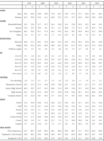
The combination of treatments from ENCOPE and controls from matched ENEUs provides several datasets. The characteristics of these working databases are presented in Table 1. These datasets are then processed according to the program evaluation techniques explained in section 4 so as to make the treatments and controls fully comparable, and the results are summarized in the next section.

4.3 Results

We apply the abovementioned methods to data for different years and groups. This allows us to test the robustness of the hypotheses on selection mechanisms. It also makes it possible to examine the evolution of the program’s impact over time. Finally it enables us to verify whether the program has differential impacts on various groups of beneficiaries.

It is important to highlight that we evaluate the impact on the probability of being employed 13 or 26 weeks after starting a training program. In addition, we evaluate the impact on wages for those who actually have a job either 13 or 26 weeks after starting training. However, given the duality of the Mexican labor

16 Since unemployment could be conjunctural (i.e., between jobs) or structural (i.e., long lasting unemployment), implicitly we are assuming that the distribution of these two types of unemployment is the same in the control and treatment groups.

(15)

[image:15.533.54.466.106.660.2]

Table 1. Descriptive statistics from selected observations from ENEU and ENCOPE

1999 2000 2001 2002 2003 2004

T C T C T C T C T C T C

Gender

Man 36.5 60.4 29.8 58.9 31.0 64.3 32.8 67.3 37.2 62.0 29.1 60.1 Woman 63.5 39.6 70.2 41.1 69.0 35.7 67.2 32.7 62.8 38.0 70.9 39.9

Kinship

Household head 18.1 23.6 12.7 23.7 16.3 25.8 16.1 25.8 18.9 25.2 16.8 24.1 Spouse 31.6 8.8 39.0 9.6 31.7 6.5 28.9 7.4 21.4 8.9 26.3 9.0 Son/ Daughter 46.5 58.5 45.1 57.4 44.2 59.5 44.2 58.7 49.9 58.4 47.5 58.9

Other 3.8 9.1 3.2 9.3 7.7 8.2 10.7 8.1 9.8 7.5 9.4 8.1

Marital Status

Married 46.0 33.1 48.1 32.9 46.6 33.3 45.9 33.4 38.4 33.8 44.1 32.8 Single 50.0 62.2 48.1 60.9 48.9 62.1 50.3 61.3 57.0 62.5 51.2 63.0 Without couple 3.5 4.7 3.8 6.2 4.5 4.6 3.8 5.3 4.7 3.8 4.7 4.1

Age

12 to 15 0.1 2.8 0.2 2.6 0.1 2.3 0.1 3.6 0.2 3.5 0.0 4.0 16 to 25 53.8 53.6 51.0 54.3 53.5 52.7 58.4 53.8 53.1 55.0 48.7 54.4 26 to 35 25.2 23.5 26.2 22.9 24.7 24.6 23.9 21.5 29.0 21.3 30.6 20.7 36 to 45 14.1 12.2 16.1 11.8 13.6 11.7 11.0 12.4 12.3 12.7 13.0 12.7 46 to 55 5.5 4.8 5.9 6.0 6.0 6.2 5.1 5.9 3.9 4.9 5.5 5.9 56 or more 1.2 3.1 0.6 2.4 2.2 2.6 1.5 2.9 1.5 2.6 2.2 2.2

Schooling

No schooling 2.0 2.3 3.1 2.1 1.3 1.8 1.0 1.8 1.1 1.9 1.4 2.2

Elementary School 28.4 22.3 27.3 19.6 23.8 19.8 24.7 21.4 14.7 21.1 17.3 19.7

Junior High School 40.9 30.7 43.7 34.1 38.6 31.4 39.0 33.8 31.3 34.9 26.4 32.8

High School 22.3 23.4 21.0 23.6 27.3 24.9 25.8 24.0 28.1 22.3 26.8 26.5 Graduate School 3.8 21.0 0.8 20.2 8.7 21.8 9.5 18.7 23.8 19.6 28.1 18.6

Region

North 13.2 32.0 30.6 31.4 20.4 32.1 18.4 34.1 21.1 24.5 17.6 18.4 Gulf 22.3 13.2 19.7 14.9 15.5 15.0 14.6 15.6 9.4 14.3 10.4 11.5 Pacific 11.6 12.3 2.7 13.5 14.1 10.6 14.7 11.1 13.9 14.5 11.1 15.5 South 13.3 7.0 5.1 6.8 10.6 6.3 15.5 6.0 11.0 5.2 7.1 7.2 Center-North 17.2 17.7 24.0 18.6 20.3 22.0 22.3 16.7 14.3 22.6 20.7 28.6

Center 12.8 9.0 5.2 8.6 11.7 7.4 7.8 10.0 10.0 9.6 8.4 8.0 Capital 9.7 8.8 12.6 6.2 7.3 6.7 6.8 6.5 20.2 9.3 24.7 10.9

Labor market

Prior Experience 54.7 86.7 44.9 86.3 48.1 89.0 58.9 88.7 71.7 87.8 62.6 86.8 Employed (+26) Formal 58.0 60.2 39.6 58.8 44.0 60.7 58.4 62.8 49.9 60.3 40.7 57.8

Employed (+26) 0.0 27.0 19.2 28.6 15.9 28.8 34.6 27.4 31.1 26.0 20.6 19.6

Source: selected observations from ENEU and ENCOPE databases (see section 4.2)

(16)

market, it is not reasonable to think that employment in the informal sector is an outcome equivalent to employment in the formal sector. Furthermore, the PROBECAT/SICAT program has different training modalities for those who seek a formal job and those who want to be self-employed. Consequently, our impact evaluation distinguishes employment and wage effects for those who took the mixed and school-based modalities, on the one hand, and for those who took the other modalities, on the other e. For the former group, finding a job in the formal sector is a success, whereas being unemployed or having an informal job is a failure. For the latter group, having a job, either formal or informal, is a success. This separation allows us to take into consideration the quality of the job as well as the type of training for a stricter impact evaluation.

Given the large array of results, we first explain the findings according to the non-parametric method that assumes selection on observables. Then, we explain the outcomes according to the parametric method that assumes selection on un-observables. We compare the results between these methods and derive insights on which method appears to give a better account of the program’s evolution. Finally, we add a section that specifically deals with the impact of the program for different program modalities and population groups.

4.4 According to the non-parametric method, assuming selection on observables

When the program to be evaluated is not implemented in a randomized way, one can resort to quasi-experimental methods to describe the impact of the program. In quasi-quasi-experimental designs, targets receiving the intervention are compared to a control group of potential targets that do not receive the intervention. To the extent that the latter resemble the intervention group on relevant characteristics and experiences, or can be statistically adjusted to resemble it, then program effects can be assessed with

Year All cases salaried Non salaried

13 weeks (1) 26 weeks (2) 13 weeks (3) 26 weeks (4) 13 weeks (5) 26weeks (6) Average Treatment effect (ATE)

1999 -13.8*** 2.8 7.5 4.9

2000 -10.6*** -0.9 -1.2*** 0.2 6.1*** 8.5***

2001 -14.8*** -12.9*** -6.1 -4.2 5.5* 4.6*

2002 3.5 3.4 29.6*** 21.9*** 19.9** 24.1***

2003 3.5 2.0 26.8*** 15.3*** 10.9 6.9

2004 -6.3** -6.4 16.5*** 27.6*** -4.3*** -1.4

Average Treatment effect on the treated (ATT)

1999 -18.1*** 0.2 6.5** 6.6

2000 -6.6** 2.1 -0.5 0.0 6.1** 10.4***

2001 -14.8*** -11.7** 3.1 -3.7 7.8** -1.8

2002 0.8 -3.1 24.5*** 11.0 13.6** 16.1**

2003 0.8 0.1 17.2*** 9.8* 3.9 14.7***

2004 -8.7* -10.2 4.7 14.9*** 1.6 1.6

[image:16.533.69.490.126.356.2]

Source: Authors’ calculations using PROBECAT, ENEU and ENECE databases.

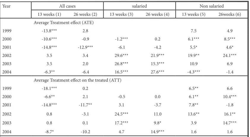
Table 2. Employment effects according to selection on observables

(17)

Year All cases salaried Non salaried 13 weeks (1) 26 weeks (2) 13 weeks (3) 26 weeks (4) 13 weeks (5) 26weeks (6) Average Treatment effect (ATE)

1999

2000 -515 *** -717 *** -613 *** -663 *** -1250 *** -900 ***

2001 -232 *** -226 ** -361 *** -463 *** -755 * -1345 ***

2002 -347 *** -432 *** -359 *** -458 *** -689 -1075 *

2003 -291 *** -317 ** -853 *** -761 *** -1197 ** NA

2004 -266 * -348 -943 *** -464 ** NA NA

Average Treatment effect on the treated (ATT) 1999

2000 -427 *** -744 *** -446 *** -660 *** -1550 *** -913 ***

2001 -339 *** -392 *** -546 *** -552 ** -671 -444

2002 -341 *** -622 *** -323 ** -523 ** -1514 -925

2003 -174 -308 -1027 *** -808 ** -648 NA

2004 -230 -580 * -1188 *** -557 * NA NA

[image:17.533.50.466.127.355.2]

Source: Authors’ calculations using PROBECAT, ENEU and ENECE databases

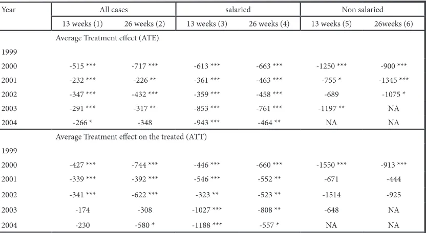
Table 3. Wage effects according to selection on observables

PROBECAT-SICAT impact on probability of employment, in pesos per month. Matching selection on observables.

a reasonable degree of confidence18_.

One way to select the control group ex-post is by using the matching method. This technique is commonly applied in evaluation research and basically consists of finding a “twin” or “partner” for each of the treated individuals. In matching design, the intervention group has already been specified. It is the evaluator’s task to construct a control group by selecting targets unexposed to the intervention that match those in the intervention group on selected characteristics. The logic of this design requires that the groups be matched in any characteristic that would cause them to differ in the outcome of interest under conditions when neither of them received the intervention. To the extent that the matching falls short of equating the groups in characteristics that will influence the outcome, selection bias will be introduced into the resulting program-effect estimate. For instance, if age is a key factor in affecting a given outcome--e.g., finding a job in three months for an unemployed person—to avoid bias, the matching of people receiving the treatment and not receiving it should be done considering, among other factors, the person’s age19_.

Once the matching is done, we can then calculate the estimated gain from the program, following Becker and Ichino’s (2002) protocol. Table 2 shows the estimated ATE and ATT for the probability of having a job after 13 and 26 weeks of starting training (i.e., after “T_o” in Graph 5) for years 1999-200420_{. The first} column shows the year analyzed, whereas columns 2 and 3 show the impact on the probability of having a job 13 and 26 weeks after starting training respectively in general (i.e., without distinguishing between the program modalities). Columns 4 and 5 show the same but for those who attended the classes for salaried

18 However, the presence of unobserved characteristics that could be related to the outcome could posit a restriction to the useful-ness of these methods.

19 For a more detailed explanation of the procedure see http://idbdocs.iadb.org/WSDocs/getdocument.aspx?docnum=907641&-Cache=True, Methodological Annex.

(18)

positions, whereas columns 6 and 7 show the same for those who attended classes for self-employment positions. The upper panel shows the ATE and the lower panel the ATT.

When we analyze the impact without distinguishing between program modalities we observe that there is a somewhat positive trend. For ATE (i.e., the expected impact for a person selected at random from the population) the estimated impact after 13 weeks of finishing training changed from a negative –13.8 percentage points in 1999 to a positive impact of 3.5 in 2003 (see column 1, upper panel, Table 2), but a negative –6.3 in 2004. In the case of 26 weeks, the figures are 2.8 and -6.4 respectively (see column 2). For this latter case, the impact was in general higher than that of 13 weeks. Similar results were found when estimating the ATT (i.e., the estimated impact for a person that actually decided to take the training) as is shown in the lower panel of the table. It should be pointed out that the results for ATE and for ATT at 13 weeks were positive in years 2002 and 2003 only (although not significantly different from zero) and at 26 weeks for all years (also not significantly positive either) except 2001.

We have also estimated the impact taking into account that there are different job qualities and modalities for the training. For the case of training the unemployed that seek a job as an employee, following columns 3 and 4 we find that the ATE is positive and significant from 2002 onwards. The ATT for 13 weeks and 26 weeks is similar. For the modality of training for self-employment (see columns 5 and 6), results are in general positive both for ATE and ATT, but significant only in some years with an irregular trend.

Table 3 shows the impact on monthly wages after 13 and 26 weeks of starting training for years 1999-2004. One striking result from this table is that all numbers that are statistically significant are negative. This means that if an average person from the population had taken the training his/ her expected wage would have been lower than if that average person had not taken the course (ATE results). Results are the same for those individuals that have actually taken the training (ATT results). The negative impact for ATE ranges from –291 pesos per month 13 weeks after finishing training in 2003, to -1345 pesos per month 26 weeks after finishing training for self-employment in year 2001. The negative impact for ATT ranges from -174 (statistically non-significant) to –1550 pesos for those that took training for self-employment in 2000. To put these numbers into context, the average impact of –232 pesos for 2001 (column 1 in Table 3) represents about 8% of the average monthly salary of a person in the respective control group. In turn, the highest expected loss of -1250 pesos for year 2000 (column 6) represents about 57% of the average monthly salary of a person in the relevant control group.

Obviously, these results of lower probabilities of finding a job, for some years, and lower wages for trainees, almost always, are so contrary to what would be expected that they beg for an explanation. Before going into it, the next section presents another way of calculating the impact of the PROBECAT-SICAT (control for unobservables) that will provide an important piece for this puzzle.

4.5 According to the parametric method, assuming selection on unobservables

(19)

Year All cases Salaried Non salaried 13 weeks (1) 26 weeks (2) 13 weeks (3) 26 weeks (4) 13 weeks (5) 26weeks (6) Average Treatment effect (ATE)

1999 13.6 *** 6.7 *** 9.1 *** 11.2 ***

2000 -18.5 *** 6.7 *** 11.4 *** 25.7 *** -2.4 *** -10.7 ***

2001 6.7 *** 22.6 *** 8.1 *** 23.3 *** 0.2 8.2 ***

2002 19.6 *** 27.6 *** 24.5 *** 39.6 *** 27.6 *** 36.0 ***

2003 2.5 *** 3.6 *** 25.8 *** 7.2 *** 67.1 *** 49.7 ***

2004 -14.9 *** -15.4 *** 2.9 *** 12.1 *** 9.3 *** 6.2 ***

Average Treatment effect on the treated (ATT)

1999 6.0 *** 2.6 *** 6.3 *** 10.0 ***

2000 -18.8 *** 6.4 *** 3.2 *** 18.2 *** -5.9 *** -14.8 ***

2001 -8.7 *** 9.8 *** -6.4 *** 6.4 *** -10.9 *** -1.9 ***

2002 12.6 *** 16.6 *** 20.1 *** 23.9 *** 12.3 *** 16.4 ***

2003 -0.3 0.9 *** 14.5 *** 3.2 *** 8.3 *** 11.9 ***

2004 -13.0 *** -13.5 *** 3.1 *** 11.4 *** -1.8 *** -4.0 ***

[image:19.533.49.465.126.356.2]

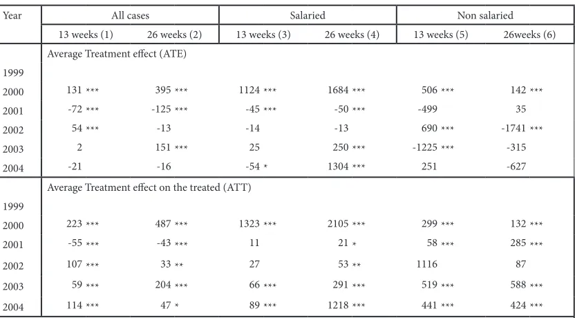
Table 4. Employment effects according to selection on un-observables

PROBECAT-SICAT impact on probability of employment, in percentage points. Regression controlling for observables.

Year All cases Salaried Non salaried

13 weeks (1) 26 weeks (2) 13 weeks (3) 26 weeks (4) 13 weeks (5) 26weeks (6) Average Treatment effect (ATE)

1999

2000 131 *** 395 *** 1124 *** 1684 *** 506 *** 142 ***

2001 -72 *** -125 *** -45 *** -50 *** -499 35

2002 54 *** -13 -14 -13 690 *** -1741 ***

2003 2 151 *** 25 250 *** -1225 *** -315

2004 -21 -16 -54 * 1304 *** 251 -627

Average Treatment effect on the treated (ATT) 1999

2000 223 *** 487 *** 1323 *** 2105 *** 299 *** 132 ***

2001 -55 *** -43 *** 11 _{21 *} _{58 ***} _{285 ***}

2002 107 *** 33 ** 27 _{53 **} 1116 87

2003 59 *** 204 *** 66 *** 291 *** 519 *** 588 ***

2004 114 *** 47 * 89 *** 1218 *** 441 *** 424 ***

Table 5. Wage effects according to selection on un-observables

[image:19.533.49.465.419.649.2]

(20)

Heckman, Tobias and Vytlacil (2001, 2003) propose a parametric method for dealing with the problem of selection on unobservables. Basically, it consists of running an econometric model for explaining the variable of interest (in our case, employment and wages) controlling for the usual observable variables (the same vector X of the previous section) and adding a variable that controls for the distribution of the unobservable variables. This distribution is assumed a priori and the validity of the procedure hinges on this assumption being correct.

In general, the procedure follows four stages. First, obtain the parameters of a probit model on the decision to take the treatment; second, compute the appropriate correction for unobservables term; third, run separate outcome-specific regressions for the treatment and control groups with appropriate unobservables-correction terms obtained from the previous step; and fourth, given the parameters of these regressions, obtain point estimates for each observation and compute the ATE and ATT parameters according to specific formulas21_.

Table 4 and Table 5 summarize the employment and wage effects, respectively, according to the parametric method assuming selection on un-observables. The employment effects for the treated (ATT) show a kind of inverted-U trend for general employment both at 13 and 26 weeks after starting training. These trends, with mostly positive and significant values can be seen both for salaried and for self-employment. This inverted-U trend means that employment effects for years 2002 and/or 2003 are significantly positive and larger effects than for previous and subsequent years. With some exceptions, the employment effects according to selection on unobservables are larger than according to selection on observables.

The wage effects for salaried workers are mostly positive and significant. Oddly, years 2000 and 2004 show sizeable positive effects for salaried workers that do not recur but look very large (more than 1,000 pesos): these would represent nearly two thirds of the monthly wage of a person in the respective control group. Wage effects for self-employed workers are usually positive and significant. The size of the positive and significant effects is also quite large (between 50% and 100% of the monthly wage of a person in the respective control group).

4.6 Comparison of results between methods

Comparing the ATE and the ATT provides information on the program’s selection mechanism, in particular on whether the program is attracting those who benefit the most from it or whether it does the opposite. Second, comparing the ATE or the ATT between methods hints at whether there is a problem of hidden bias. Finally, comparing results for each method over time allows us to ascertain whether there is a program impact robust to evaluation methods and data collection period.

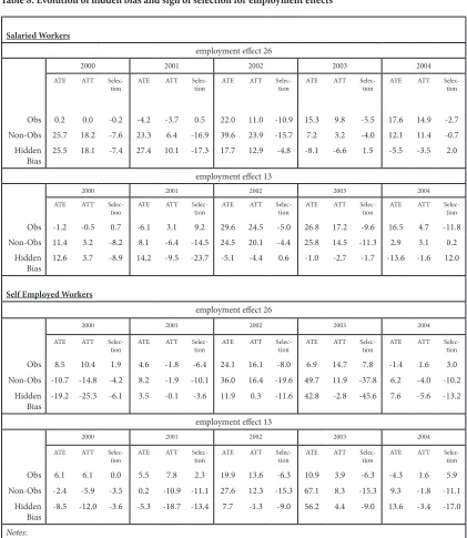
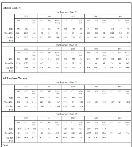
Table 6 to Table 9 summarize the results of our estimations with a compilation of the employment and wage ATE and ATT, distinguishing two methods and two types of workers: salaried and self-employed. One main conclusion can be derived from each table. The employment effect of the program on the treated (ATT) is significantly positive, according to both methods, for salaried as well as self-employed workers in most of the years considered (see Table 6). On the other hand, wage effects vary radically by method, as well as by period and type of worker (Table 7).

With respect to employment effects, there are several regularities we would like to highlight. First, for salaried workers, the difference in estimates assuming selection on observables and selection on unobservables declines from large and positive in 2000 to small and negative in 2004 (see Table

(21)

28

M

ar

ce

lo D

el

aj

ara, Sa

m

ue

l F

rei

je a

n

d I

sidr

o S

olo

aga

Weeks after starting training: 1999 2000 2001 2002 2003 2004

13 26 13 26 13 26 13 26 13 26 13 26

Average Treatment effect (ATE)

Assuming selection-on-observables (non-parametric)

Salaried NA NA -1.2 0.2 -6.1*** -4.2 29.6*** 21.9*** 26.8*** 15.3*** 16.5*** 17.6*** (1.6) (2.2) (1.7) (2.9) (3.5) (4.5) (2.8) (3.8) (3.6) (3.8) Self-employed 7.5 4.9 6.1*** 8.5*** 5.5* 4.6* 19.9** 24.1*** 10.9 6.9 -4.3*** -1.4 (5.2) (4.8) (1.9) (1.4) (3.1) (2.8) (8.5) (7.0) (11.2) (5.7) (1.6) (3.8) Assuming selection on observables (non parametric)

salaried NA NA 11.4*** 25.7*** 8.1*** 23.3*** 24.5*** 39.6*** 25.8*** 7.2*** 2.9*** 12.1*** (0.1) (0.1) (0.4) (0.3) (0.2) (0.3) (0.3) (3.0) (2.0) (0.3) Self employed 9.1*** 11.2*** -2.4*** -10.7*** 0.2 8.2*** 27.6*** 36.0*** 67.1*** 49.7*** 9.3*** 6.2***

(0.2) (0.2) (0.2) (0.3) (0.5) (0.5) (0.4) (0.6) (0.5) (0.8) (4.0) (0.6) Average Treatment effect on the treated (ATT)

Salaried NA NA -0.5 0.04 3.1 -3.7 24.53*** 11.02 17.2*** 9.8* 4.7 14.9*** (2.3) (2.6) (3.2) (3.7) (5.5) (6.9) (3.4) (5.1) (5.3) (5.7)

Self-employed 6.5*** 6.6 6.1** 10.4*** 7.8** -1.8 13.6** 16.1** 3.9 14.7*** 1.6 1.6 (3.0) (4.1) (3.0) (1.6) (3.9) (2.3) (5.6) (6.6) (6.5) (5.1) (3.8) (7.9)

Assuming selection on observables (non parametric)

salaried NA NA 3.2*** 18.2*** -6.4*** 6.4*** 20.1*** 23.9*** 14.5*** 3.2*** 3.1*** 11.4*** (0.1) (0.1) (0.3) (0.4) (0.3) (0.3) (0.4) (0.4) (0.4) (0.3) Self employed 6.3*** 10.0*** -5.9*** -14.8*** -10.9*** -1.9*** 12.3*** 16.4*** 8.3*** 11.9*** -1.8*** -4.0***

[image:21.533.94.699.118.458.2]

(22)

29

E

va

lu

atio

n o

f t

ra

inin

g f

or t

he un

em

plo

ye

d in M

exico: le

ar

nin

g b

y co

m

pa

rin

g m

et

ho

ds

Weeks after starting training: 1999 2000 2001 2002 2003 2004

13 26 13 26 13 26 13 26 13 26 13 26

Average Treatment effect (ATE)

Salaried NA NA -613*** -663*** -361*** -463*** -359*** -458*** -853*** -761*** -943*** -464

(112) (133) (122) (164) (107) (160) (195) (245) (223) (212)

Self-employed NA NA -1250*** -900*** -755* -1345*** -689 -1075* -1197** NA NA NA

(238) (219) (420) (420) (785) (594) (520) Assuming selection on observables (non parametric)

salaried NA NA 1124*** 1684*** -45*** -50*** -14 -13 25 250*** -54* 1304

(24) (28) (9) (16) (19) (19) (28) (28) (31) (74)

Self employed NA NA -51 -112*** -824*** -782*** 690*** -1741*** -1225*** -315** 251** -627

(39) (26) (65) (75) (93) (98) (133) (129) (125) (142)

Average Treatment effect on the treated (ATT) Assuming selection-on-observables (non-parametric)

Salaried NA NA -466*** -660*** -546*** -522** -323** -523** -1027*** -808** -1188*** -557

(121) (149) (170) (222) (154) (243) (248) (373) (338) (307)

Self-employed NA NA -1550*** -913*** -671 -444 -1514 -925 -648 NA NA NA

(355) (330) (657) (685) (1048) (901) (832) Assuming selection on observables (non parametric)

salaried NA NA 1323*** 2105*** 11 21* 27 53** 66*** 291*** 89*** 1218

(24) (29) (10) (12) (17) (21) (19) (30) (28) (88)

Self employed NA NA 299*** 132*** 58 285*** 1116*** 87 519*** 588*** 441*** 424

(23) (17) (58) (52) (118) (98) (92) (123) (75) (75)

[image:22.533.59.653.110.453.2]

(23)

Salaried Workers

employment effect 26

2000 2001 2002 2003 2004

ATE ATT Selec-tion

Obs 0.2 0.0 -0.2 -4.2 -3.7 0.5 22.0 11.0 -10.9 15.3 9.8 -5.5 17.6 14.9 -2.7 Non-Obs 25.7 18.2 -7.6 23.3 6.4 -16.9 39.6 23.9 -15.7 7.2 3.2 -4.0 12.1 11.4 -0.7

Hidden Bias

25.5 18.1 -7.4 27.4 10.1 -17.3 17.7 12.9 -4.8 -8.1 -6.6 1.5 -5.5 -3.5 2.0

2000 2001 2002 2003 2004

ATE ATT Selec-tion

Obs -1.2 -0.5 0.7 -6.1 3.1 9.2 29.6 24.5 -5.0 26.8 17.2 -9.6 16.5 4.7 -11.8 Non-Obs 11.4 3.2 -8.2 8.1 -6.4 -14.5 24.5 20.1 -4.4 25.8 14.5 -11.3 2.9 3.1 0.2

Hidden Bias

12.6 3.7 -8.9 14.2 -9.5 -23.7 -5.1 -4.4 0.6 -1.0 -2.7 -1.7 -13.6 -1.6 12.0

Self Employed Workers

2000 2001 2002 2003 2004

ATE ATT Selec-tion

Obs 8.5 10.4 1.9 4.6 -1.8 -6.4 24.1 16.1 -8.0 6.9 14.7 7.8 -1.4 1.6 3.0 Non-Obs -10.7 -14.8 -4.2 8.2 -1.9 -10.1 36.0 16.4 -19.6 49.7 11.9 -37.8 6.2 -4.0 -10.2

Hidden Bias

-19.2 -25.3 -6.1 3.5 -0.1 -3.6 11.9 0.3 -11.6 42.8 -2.8 -45.6 7.6 -5.6 -13.2

2000 2001 2002 2003 2004

ATE ATT Selec-tion

Obs 6.1 6.1 0.0 5.5 7.8 2.3 19.9 13.6 -6.3 10.9 3.9 -6.3 -4.3 1.6 5.9 Non-Obs -2.4 -5.9 -3.5 0.2 -10.9 -11.1 27.6 12.3 -15.3 67.1 8.3 -15.3 9.3 -1.8 -11.1

Hidden Bias

-8.5 -12.0 -3.6 -5.3 -18.7 -13.4 7.7 -1.3 -9.0 56.2 4.4 -9.0 13.6 -3.4 -17.0

Notes:

Hidden bias is the difference between the estimates assuming selection on unobservables minus the estimates assuming selection on observables.

Selection is the difference between ATT and ATE.

[image:23.533.45.466.102.587.2]

(24)

8, row entitled “hidden bias”). This means that up to year 2002, there was an important “hidden bias” and, hence, assuming selection on observables could be misleading. An interpretation of this “hidden bias” could be that individuals who participate in the program exert, on average, less effort in looking for a job than individuals who do not participate. Therefore, when not controlling for this unobservable variable, the matching method is not taking into account the fact that participants use less effort (or some other unobservable variable that is associated with lower employment rates). Again, this hidden bias appears to decline from 2002 onwards and both methods show similar results in 2003 and 2004.

Second, the difference between the ATT and the ATE for salaried workers according to both methods is mostly negative, but is usually greater in year 2001 or 2002 than in other years. These years represent important changes in the program. Particularly, the school-based modality was phased out and the mixed modality was enhanced (see Graph 4). Since a positive difference between ATT and ATE mean a positive selection mechanism (i.e., those with greater expected benefits from the program are also those with a higher probability of entering the program), then it seems that the decline in the negative selection (observed under both methods) portrays an indication that program modifications induce a better targeting in its use. This is because the concentration of the program in the mixed modality (with its requirement that firms should hire 80% of the trainees) ought to be associated with an increasing employment impact (seen in both methods) and better selection (i.e., those who would benefit most from it are more likely to select it). The greater impacts of the program in 2002, 2003 and 2004 can also be associated with the concentration on the mixed modality.

With respect to the self-employed, the effect on the treated (ATT) according to selection on unobservables varies from negative in years 2000 and 2001, to positive in 2002-2003 and negative again in 2004. These results are accompanied by a negative selection mechanism (see Table 8, lower panel). This seems to indicate that the self-employment and productive project modalities attract individuals who benefit less from the program (perhaps, those who find it very difficult to become self-employed by themselves), but occasionally help them. A similar trend is observed according to selection on observables, but with mostly positive results. The trend of the hidden bias and the selection effect differs across methods and over time, so no clear pattern can be recognized.

The wage effects, as mentioned earlier, differ by method of estimation. Table 3 shows that wage effects on the treated (ATT) are negative for all workers every year when assuming selection on observables. On the other hand, these effects are usually positive if assuming otherwise (see Table 5). Table 9 shows that, in the case of salaried workers, there is a positive and large hidden bias. This hidden bias is often as large as the negative wage effect reported by selection on observables. Consequently, the wage effect on the treated for the salaried is generally positive and small (this is less than 100 pesos a month)22_{. In the case of self-employed workers, the hidden bias varies in} sign and size. Notwithstanding this, the wage effect on the treated is always positive but fluctuates wildly in size. Given the instability of results, it appears that the program does not have a robust and steady impact so its wage effects upon those in salaried employment or who are self-employed are somewhat haphazard.

(25)

Salaried Workers

2000 2001 2002 2003 2004

ATE ATT Selec-tion

ATE ATT Selec-tion(2)

ATE ATT Selec-tion

Obs -663 -660 3 -463 -552 -89 -458 -523 -65 -761 -808 -47 -464 -557 -93

Non-Obs 1684 2105 422 -50 21 70 -13 53 66 250 291 41 1304 1218 -86

Hidden Bias

2347 2765 419 413 572 159 445 576 131 1011 1099 88 1768 1775 7

2000 2001 2002 2003 2004

ATE ATT Selec-tion

Obs -613 -446 167 -361 -546 -185 -359 -323 36 -853 -1027 -174 -943 -1188 -245

Non-Obs 1124 1323 199 -45 11 56 -14 27 41 25 66 41 -54 89 143

Hidden Bias

1737 1769 32 316 557 240 345 350 5 878 1093 215 889 1277 388

Self Employed Workers

2000 2001 2002 2003 2004

ATE ATT Selec-tion

Obs -900 -913 -13 -1345 -444 901 -1075 -925 150

Non-Obs -112 132 244 285 -782 -1067 -1741 87 1828 -315 588 903 -627 424 -1051

Hidden Bias

788 1045 257 1630 -338 -1968 -666 1012 1678

2000 2001 2002 2003 2004

ATE ATT Selec-tion

Obs -1250 -1550 -300 -755 -671 -689 -1514 -825 -1197 -648 549

Non-Obs -51 299 351 58 -824 -882 690 1116 426 -1225 519 1744 251 441 -190

Hidden Bias

1199 1849 651 812 -153 -882 1379 2630 1251 -28 1167 1195

Notes:

Hidden bias is the difference between the estimates assuming selection on unobservables minus the estimates assuming selection on observables.

Selection is the difference between ATT and ATE.

[image:25.533.42.467.108.579.2]

(26)

1999 2000 2001 2002 2003 2004

Modality 13 26 13 26 13 26 13 26 13 26 13 26

School- based -6.2*** -32.4*** -3.8*** -26.5*** -1.4 -36.4*** (0.4) (0.5) (0.1) (0.2) (3.4) (2.8)

Mixed 15.1*** 11.9*** 22.5*** 23.4*** 29.7*** 26.0*** 20.8*** 15.1*** 22.5*** 16.9*** (0.7) (0.7) (0.5) (0.5) (1.9) (1.9) (0.7) (0.6) (0.5) (0.6)

MyPEs(3) _1.4** _-8.7*** _0.4 _-4.4*** _-3.4* _-14.5*** _2.9*** _6.4*** _3.8*** _9.9***

(0.6) (0.6) (0.3) (0.4) (1.8) (1.7) (0.7) (0.8) (0.6) (0.8)

Self - employment(4) _-8.6*** _-16.2*** _-10.2*** _-22.4*** _-4.7** _-15.7*** _-2.0*** _-0.2 _-18.6*** _-13.7*** _-17.5*** _-10.7***

(0.5) (0.5) (0.2) (0.2) (2.3) (1.7) (0.7) (0.8) (1.0) (0.7) (1.0) (1.4)

ILE(5) _NC _NC _NC _NC _NA _NA

Basic skills 5.3*** -34.2*** -6.9*** -17.9*** NA NA (1.7) (1.5) (0.5) (0.8)

Sinorcom(6) _-6.9*** _-30.9*** _-14.0*** _-25.8*** _NA _NA

(1.4) (1.34) (0.3) (0.3)

Health sector 19.4*** 14.1*** -20.2*** 0.4 NA NA (2.0) (2.2) (3.8) (2.9)

Bouchers for training -29.0*** -18.1*** -27.5*** -19.2*** (1.0) (1.0) (0.6) (0.7)

Unemployed with Technical or professional skills

-18.9*** 16.5*** -19.6*** -20.8***

(2.0) (1.4) (0.6) (0.7)

Based on technical norms for labor training

10.5*** 14.2***

(0.9) (1.1)

Lock out -39.5*** -28.2**

(9.4) (11.4)

Capacity training 28.2*** 21.7***

(1.4) (0.9)

On the job training -0.1 3.4***

(0.9) (0.9)

Productive training -26.4*** -17.9***

(0.9) (1.3)

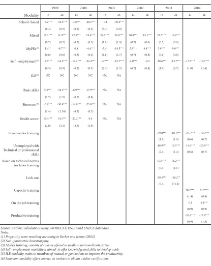
Source: Authors’ calculations using PROBECAT, ENEU and ENECE databases. Notes:

(1) Propensity score matching according to Becker and Ichino (2002). (2) Non- parametric bootstrapping.

[image:26.533.72.487.146.669.2]

(3) MyPEs training, consists of courses offered in medium and small enterprises. (4) Self - employment modality is aimed to offer knowledge and skills to develop a job. (5) ILE modality trains to members of mutual or ganizations to improve the productivity. (6) Sinorcom modality offers courses to workers to obtain a labor certification. Table 10. Employment ATT by modality

Treatment on the Treated Effect (TT) By Modalities

Assuming selection on unobservables:Parametric Method (1)

(27)

2000 2001 2002 2003 2004

Modality 13 26 13 26 13 26 13 26 13 26

School- based 108*** 168*** 16 -5 (16) (21) (87) (136)

Mixed 49*** 80*** 60* 45 81*** 82*** 77*** 183*** (15) (17) (33) (32) (19) (21) (27) (34) MyPEs(3) _443*** ₄₇ ₈₅ ₅₈ ₄₁ _52* _63** _90***

(20) (14) (53) (42) (29) (31) (25) (33)

Self - employment(4) ₂ _16* ₁₂₄ ₁₂ _-31 _-89 ₁₀₇ _161** _-7 ₁₆

(9) (9) (129) (62) (67) (56) (87) (79) (153) (96) ILE(5) _NC _NC _NA _NA

Basic skills 2741*** 74 NA NA (201) (39)

Sinorcom(6) _59*** ₂₈ _NA _NA

(23) (23)

Health sector 6 42 NA NA (76) (82)

Bouchers for training 147 151 1 621*** (221) (122) (221) (167) Unemployed with

Technical or professional skills

563 421** 342 204 (345) (206) (236) (141)

Based on technical norms for labor training

177*** 215*** (42) (48)

Lock out

Capacity training 130*** 154***

(43) (47)

On the job training 46 226***

(42) (61)

Productive training -36 -43

(219) (149)

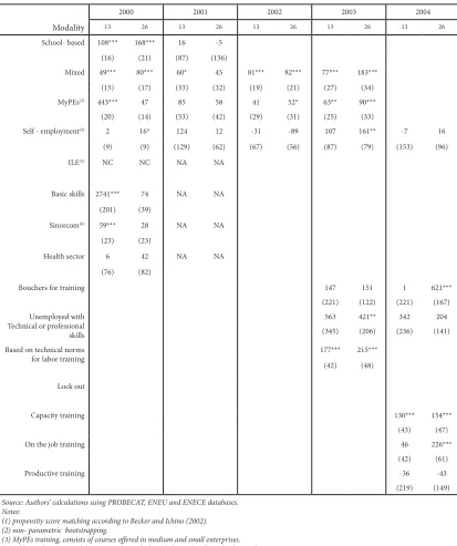
Source: Authors’ calculations using PROBECAT, ENEU and ENECE databases. Notes:

(1) propensity score matching according to Becker and Ichino (2002). (2) non- parametric bootstrapping.

[image:27.533.49.462.151.644.2]

(3) MyPEs training, consists of courses offered in medium and small enterprises. (4) Self - employment modality is aimed to offer knowledge and skills to develop a job. (5) ILE modality trains to members of mutual or ganizations to improve the productivity. (6) Sinorcom modality offers courses to workers to obtain a labor certification. Table 11. Wage ATT by modality

Treatment on the Treated Effect (TT) By Modalities

Assuming selection on unobservables: Parametric Method(1)