Investigating Diesel Engine Performance and Emissions Using CFD

Investigating Diesel Engine Performance and Emissions

Using CFD

Tarek M. Belal1, El Sayed M. Marzouk2, Mohsen M. Osman1 1_{Department of Mechanical Engineer, Alexandria University, Alexandria, Egypt} 2_{Department of Mechanical Engineering, Umm Al-Qura University, Makka, KSA}

Email: tarek.belal@eg.bureauveritas.com, emmarzouk@yahoo.com, mohsen7351@yahoo.com

Received November 23, 2012; revised December 22, 2012; accepted January 7, 2013

ABSTRACT

Fluid flow in an internal combustion engine presents one of the most challenging fluid dynamics problems to model. This is because the flow is associated with large density variations. So, a detailed understanding of the flow and com- bustion processes is required to improve performance and reduce emissions without compromising fuel economy. The simulation carried out in the present work to model DI diesel engine with bowl in piston for better understanding of the in cylinder gas motion with details of the combustion process that are essential in evaluating the effects of ingesting synthetic atmosphere on engine performance. This is needed for the course of developing a non-air recycle diesel with exhaust management system [1]. A simulation was carried out using computational fluid dynamics (CFD) code FLU- ENT. The turbulence and combustion processes are modeled with sufficient generality to include spray formation, delay period, chemical kinetics and on set of ignition. Results from the simulation compared well with that of experimental results. The model proved invaluable in obtaining details of the in cylinder flow patterns, combustion process and combustion species during the engine cycle. The results show that the model over predicting the maximum pressure peak by 6%, (p-θ), (p-v) diagrams for different engine loads are predicted. Also the study shows other engine parame- ters captured by the simulation such as engine emissions, fuel mass fraction, indicated gross work, ignition delay period and heat release rate.

Keywords: Numerical Simulation; Unsteady Flow; Combustion; Diesel Engine

1. Introduction

The requirement to meet the challenge of producing cleaner and more efficient power plants will intensify further over the next few years. This challenge requires an increased commitment to research by the transporta- tion industry. The internal combustion engine represents one of the more challenging fluid mechanics problems to model because the flow is compressible with large den- sity variations, relatively high Mach number, turbulent, unsteady, cyclic, and non-stationary, both spatially and temporally. Much progress has been made in CFD model development for engines in recent years.

Clean diesel engines are one of the fuel efficient and low emission engines of interest in the automotive Indus- try. The combustion chamber flow field and its effect on fuel spray characteristics plays an important role in im- proving the efficiency and reducing the pollutant emis- sion in a direct injection diesel engine, in terms of influ- encing processes of breakup, evaporation mixture forma- tion, ignition, combustion and pollutant formation. CFD modeling is a valuable tool to acquire detailed informa- tion about these important processes. In this context [2],

the characteristics of ultra-high injection pressure diesel fuel sprays are simulated and validated in a quiescent constant volume chamber. A profile function is utilized in order to apply variable velocity and mass flow rate at the nozzle exit. The CFD model is also applied to an open cycle engine model to study the effects of engine flow field features such as swirl and tumble motions on the spray behavior [2].

A multi-zone direct-injection (DI) diesel combustion model has been implemented for full cycle simulation of a turbocharged diesel engine [3]. The above combustion model takes into account the following features of the spray dynamics:

 the detailed evolution process of fuel sprays;

 interaction of sprays with the in-cylinder swirl and the walls of the combustion chamber;

 the evolution of a Near-Wall Flow (NWF) formed as a result of a spray-wall impingement as a function of the impingement angle and the local swirl velocity;

 interaction of Near-Wall Flows formed by adjacent sprays;

ration rate in the spray and NWF zones.

A NOx calculation sub-model uses detailed chemistry analysis which considers 199 reactions of 33 species. A soot formation calculation sub-model used is the phe- nomenological one and takes into account the distribu- tion of the Sauter Mean Diameter in injection process. The ignition delay sub-model implements two concepts. The first concept is based on calculations using the con- ventional empirical equations. In the second approach the ignition delay period is estimated using relevant data in the calculated comprehensive 4-D map of ignition delays. The model has been validated using published experi- mental data obtained on high- and medium-speed engines. Comparison of results demonstrates a good agreement between theoretical and experimental sets of data [3].

By separating the fluid dynamic calculation from that of the chemistry, the unsteady flamelet model allows the use of comprehensive chemical mechanisms, which in- clude several hundred reactions. This is necessary to de- scribe the different processes that occur in a DI Diesel engine such as auto ignition, the burnout in the partially premixed phase, the transition to diffusive burning, and formation of pollutants like NOx and soot. The experi- mental results show good agreement for the whole com- bustion cycle (ignition delay, maximum pressures, torque and pollutant formation) between the two-component ref- erence fuel and Diesel. The simulations are performed for both reference fuels and are compared to the experi- mental data. Pollutant formation (NOx and soot) is pre- dicted for both reference fuels. The contributions of the different reaction paths (thermal, prompt, nitrous, and re- burn) to the NO formation are shown. Finally, the im- portance of the mixing process for the prediction of soot emissions is discussed [4].

The KIVA code is widely used for model development in academia due to the availability of the source. How- ever, its capability for resolving complex geometries is limited.

The KIVA engine simulation developed by Los Ala- mos National Laboratory was used to characterize the combustion of alternative fuels in a direct injection diesel engine. Rapeseed oil, its methyl ester and hexadecane were used in engines run at 3000 rev/min and 50% maxi- mum torque. Approximately 40 consecutive cycles were phase averaged to derive the pressure traces for com- parison to KIVA predictions. The engine parameters and the fuel properties used in the simulations are described. Simulation results were good for the methyl ester and for hexadecane which was used as a reference fuel. The mo- del predicted lower pressures for the rape oil than those which were experimentally observed [5].

A modified CFD code based on the KIVA family of codes incorporating several strategies for reducing the computational time required for diesel engine simulations

is presented. The improved code and coarse meshes are used together to simulate combustion in a heavy-duty Mitsubishi Heavy Industries diesel engine operated over a range of loads, speeds, and injection strategies. The av- erage simulation time from IVC to EVO is reduced from around 60 hours to 1 hour through the use of 12 proces- sors and the new strategies [6].

On the other hand, other commercial CFD codes such as STAR-CD, FIRE, VECTIS and FLUENT are frequently used by industry due to their superior mesh generation interfaces and because of their available user support. Some scientists combined STAR-CD and KIVA code for the engine simulations but they concluded that, it would be preferable to implement the advanced sub models di- rectly into one commercial code for engine simulations [7].

The gas motion inside the engine cylinder plays a very important role in determining the thermal efficiency of an internal combustion engine. A better understanding of in cylinder gas motion will be helpful in optimizing en- gine design parameters. An attempt has been made to study the combustion processes in a compression ignition engine and simulation was done using computational fluid dynamic (CFD) code FLUENT, Turbulent flow modeling and combustion modeling was analyzed in formulating and developing a model for combustion process [8].

This paper describes the development and use of sub models for combustion analysis in direct injection (DI) diesel engine. In the present study the Computational Fluid dynamics (CFD) code FLUENT is used to model complex combustion phenomenon in compression igni- tion (CI) engine. The results obtained from modeling were compared with experimental investigation. Conse- quences in terms of pressure, rate of pressure rise and rate of heat release are presented. The rate of pressure rise and heat release rate were calculated from pressure based statistics. The modeling outcome is discussed in detail with combustion parameters. The results presented in this paper demonstrate that, the CFD modeling can be the reliable tool for modeling combustion of internal com- bustion engine [9].

2. Scope of Present Work

3. Mathematical Description

3.1. Mesh and Boundaries

The mathematical models in CFD start with combustion chamber geometry approximation representation (engine mesh) and boundaries types. The geometry can be made using the pre-processor as shown in Figure 1. The gam-

bit software (pre-processor is used to build and meshing a model [10]. Table 1 shows engine data [11,12].

3.2. Numerical Modeling

[image:3.595.61.287.293.540.2]

The physical phenomena of combustion flows in internal combustion engines are very complex, this study uses Eu- lerian and Lagrangian equations in Fluent code to solve the gas and liquid phase’s governing equations [10]. The gas governing equations consist of mass, momentum,

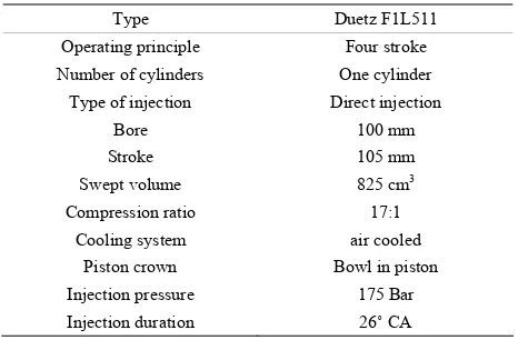
Figure 1. Engine combustion chamber mesh. Table 1. F1L511 Engine Data.

Type Duetz F1L511

Operating principle Four stroke Number of cylinders One cylinder

Type of injection Direct injection

Bore 100 mm

Stroke 105 mm

Swept volume 825 cm3

Compression ratio 17:1 Cooling system air cooled

Piston crown Bowl in piston Injection pressure 175 Bar Injection duration 26˚ CA

energy, species, turbulent equation, and chemical reac- tion. The liquid fuel governing equations contain the equation of motion, the droplet energy, and spray equa- tions. Regarding the physical boundary conditions, velo- city at wall is approximated by turbulent law-of-the-wall velocity and temperature at wall prescribed by fixed tem- perature (cylinder head = 490 K, cylinder wall = 473 K and piston and piston bowl = 550 K. The program starts at CA = 239˚ CA at inlet valve close with inlet charge already fill the cylinder and ends at CA = 469˚ CA at ex- haust valve opening. That means the simulation is count- ing for the indicated gross work and associated combus- tion parameters. The simulation is based on the experi- mental work using the DI diesel engine F1L511 [13]. The present model uses standard k-ε model for solving Navier stokes equations employing the eddy dissipation concept.

3.2.1. Modeling Basic Fluid Flow

It is often required to model a region of the engine as an open thermodynamic system. Such model is appropriate when the gas inside the open system boundary can be assumed uniform in composition and state at each point in time, and when that state and composition vary with time due to heat transfer, work transfer, mass flow across the boundary, and boundary displacement. Governing equations are mass, momentum equations and energy equations. These equations for open system, with time or crank angle as the independent variable, are the building blocks for thermodynamic based models.

Continuity equation:

 

Sm

t

 _ 

   

 v (1)

Momentum equation:

 





p

 

t    



         

 v vv g F (2)

3.2.2. Heat Transfer Modeling

The energy equation solved is taking the following form:

 









 



eff j j j eff



h

E E p

t

k T h S

 



 _{   }



   



  

v

J v

(3) 

The first three terms on the right-hand side of Equation (3) represent energy transfer due to conduction, species diffusion, and viscous dissipation, respectively. Sh includes

the heat of chemical reaction, and any other volumetric heat sources may be defined.

3.2.3. k-ε Model

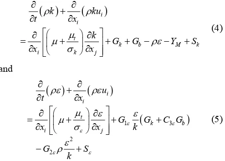
[image:3.595.56.289.584.737.2]

empirical model, and the derivation of the model equa- tions rely on phenomenological considerations and em- piricism [14].





 



i



i

t

k b

i k j

k ku t x k G G x x      _         _   _     

   YM Sk

(4)

and

 









1 k 3 b

G G C G

k    2 2 i i t i j u t x x x G S k                       _   _         (5)

3.2.4. Combustion Modeling

The ignition/combustion model is based on a modified eddy dissipation concept (EDC) which has been imple- mented into the CFD code. Multiple simultaneous chemi- cal reactions can be modeled, with reactions occurring in the bulk phase (volumetric reactions) and/or on wall sur- faces. The conservation equation takes the following ge- neral form:

 

Yi



Yi



i Ri S

t  

 _{       }

 v J

2 2

H O N

c

h j

 

 

 

2 N NO

O NO

i (6)

It is assumed that reaction occurs in small turbulent structures, called the fine scales [15]. The bulk reaction is assumed to be:



2 2



2 2

C H O N

H CO CO

n m

a b

e f g

    

Zeldovich mechanisms [8]:

2

O N

O N

N OH H NO

         2 2 H O N 2OH CO O 2OH        The equilibrium reactions are:

2 2 2 2 2 2 H 2 O 2 N 2 O H CO O H O O

  

3.2.5. Engine Ignition Modeling

For the present study the Auto-ignition model (Harden- burg model) [16] is the most suitable one for simulating direct injection Diesel engine. The transport equation for an ignition species, Yig is given by:

ig t

ig ig ig

t

Y

Y Y S

t Sc

 _  _

  

     _  _

 v _{ } (7)

The ignition delay period is calculated using the Har- denburg and Hase correlation [9] which is given by:

1 0.22 _exp 1 1 21.2

6 17,190 12.4

p id e p a C S E

N RT p

          _ _  _  __{ }             (8)

3.2.6. Discrete Phase Modeling

The Lagrangian discrete phase’s model in the CFD code follows the Euler-Lagrange approach. For x-direction it takes the following form









d d

x p p

D p x

p g u

F u u F

t        





(9)

3.2.7. Spray Modeling

In the present study the collision model along with the TAB breakup model are used [17-19].

f

crit 1 2

2.4 min 1.0

b r r

We     _  _  





(10)





2

2 d d n

n c

y t

A y We



 

 

  

 

  (11)

3.2.8. Emissions Modeling

In the present study the mass transport equation for the NO species is solved, taking into account convection, diffusion, production and consumption of NO and related species.



YNO





YNO





D YNO



SNO

t   



       

 v (12)

For soot formation the two-step Tesner model is used [20]. The model predicts the generation of radical nuclei and then computes the formation of soot on these nuclei.









t

nuc nuc nuc nuc

nuc

b b b R

t                 _  _

 v _{ }

soot soot,form soot,comb

R R R

(13)

  (14)

4. Results and Analysis

4.1. Grid Analysis

The computational grids of the DI diesel engine are showed in Figure 1. The present study model is build us-

[image:4.595.58.290.127.293.2]

zones. The first zone is the cylinder zone and the second is the bowl zone. The first zone uses the hexagonal cells and the second zone uses tetrahedral cells as shown in

Figure 1. In engine operation, valves and the piston move,

so the mesh should move according to the real engine in order to simulate the charge of valve and piston position with crank angle. Piston and piston bowl movement are decided by the stroke, connecting rod and crank angle. Simulation starts at 239˚ CA and ends at 469˚ CA. This is the period from the inlet valve closing till exhaust valve opening. That means thermodynamically; the com- pression stroke and power stroke only accounted in this study (indicated gross work). The simulation time step is 0.5 crank angles. Each computer run spends about 12 hours on IBM compatible computer using quad duo pro- cessor with 2 GHz and 4 MB cache and 6 GB RAM. The simulation uses fixed temperature boundary conditions [21] and the initial conditions driven from the experi- mental work [13].

4.2. Model Validation

Figure 2 shows the comparison of the measured and pre-

dicted cylinder pressures. The ignition model scaling fac- tor tuned for the first case (maximum load simulation) and kept constant in all cases (other load simulated). The ignition point in most cases is nearly captured. The peak pressure and the pressure gradient over the combustion period produced by CFD simulation match closely with measurements. The peak cylinder pressure is over predi- cated by about 6%. Figures 3-6 demonstrate the in-cyl-

inder processes reproduced by CFD simulation using a series of distribution plots illustrating temperature, pres- sure, fuel mass fraction and gas velocity across the cyl- inder center plan respectively.

4.3. Engine Performances

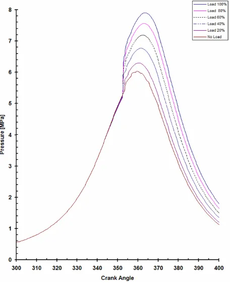
The engine performance at different loads is shown in

Figure 7. The figure shows the predicted performance

from maximum load till the no load. From the pressure- crank angle diagram the peaks pressure at different loads are determined, also the start of injection, start of ignition is observed. Figure 8 shows p-v diagram which is not

closed, because the simulation period did not reach to the end of expansion stroke at exhaust valve opening.

Figure 9 shows predicted rate of heat release. The

curve accurately and clearly determined the different com- bustion zones and delay time period.

The start of injection crank angle is determined from [13] and the injection period is determined from [11,12]. The delay time period is determined to be from the start of injection till the p-θ change its slope as identified in

Figure 9. This period is nearly 11 crank angles vary ac-

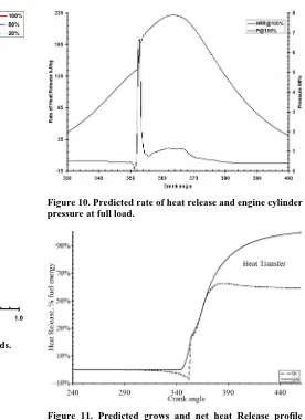
cording to the φ (equivalence ratio) or load. Figure 10

Figure 2. Comparison of the measured and predicted in- cylinder pressures.

Figure 3. Temperature distribution in (K) at φ = 0.556, CA = 339 (maximum load).

shows the predicted heat release along with the predicted engine pressure at maximum load. From Figure 10 we

[image:6.595.65.537.80.281.2] [image:6.595.57.292.83.284.2]

Figure 4. Pressure distribution in (Bar) at φ = 0.556, CA = 339 (maximum load).

Figure 5. C10H22 mass fraction at φ = 0.556, CA = 345

(maximum load).

[image:6.595.309.538.83.282.2]

magnitude of the gross and net heat release, heat transfer and heat of vaporization and heating up of the fuel at 1500 RPM for the base line engine. The heat release an- alysis method [23] is used to obtain the combustion in- formation from the pressure data. The net heat release is the gross heat release due to combustion extracts from it, the heat transfer to the walls (omitting the crevice effect) and the effect of fuel vaporization and heat up. The energy change associated with heating up fuel vapor from injec- tion temperature to typical compression air temperature is about 6% of the fuel heating value. The heat transfer integrated over the duration of the combustion period is about 35% of the total heat release. The small kink in the lower part of the curve shows the heat of vaporization

Figure 6. Gas velocity magnitude (m/s) at φ = 0.556, CA = 339 (maximum load).

Figure 7. Pressure-crank angle at different engine loads. and heating up fuel.

Figure 12 shows the predicted temperature-crank an-

gle diagram at different loads. The curve shows that in- creasing the load which corresponding to increasing the fuel mass flow rate results in increasing the combustion temperature. Figure 12 shows that the temperature of the

[image:6.595.310.538.320.603.2] [image:6.595.58.287.320.532.2]

[image:7.595.265.541.76.456.2] [image:7.595.57.284.77.407.2]

Figure 8. Pressure-volume diagram at different loads.

Figure 9. Predicted rate of heat release diagram identifying different diesel combustion phases at maximum load. jection crank angle represent the interaction between the liquid fuel (heated up) and the air in the cylinder (cooled).

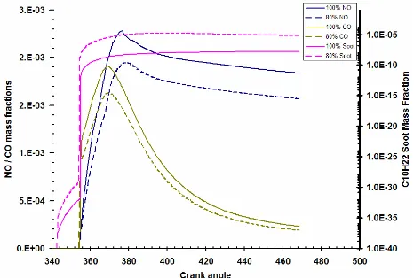
4.4. Emissions

Engine emissions due to combustion of hydrocarbon fuel depend on the combustion equations and the emission model solved to calculate engine pollutant. In the present study the combustion emissions CO, CO2, NO and Soot

are calculated. Figure 13 shows NO concentrations rise

from the residual gas value following the start of com- bustion, to a peak at the point where the burned gas equi-

[image:7.595.59.285.401.559.2]

Figure 10. Predicted rate of heat release and engine cylinder pressure at full load.

Figure 11. Predicted grows and net heat Release profile during combustion at 1500 RPM.

Figure 12. Temperature-crank angle diagram. valence ratio changes from rich to lean (where the CO and CO2 concentration has its maximum value).

[image:7.595.309.539.475.643.2]

[image:8.595.56.289.85.242.2]

Figure 13. Concentration of Soot, NO and CO for different loads as a function of crank angle.

5. Conclusions

From the present study the main conclusions are:

 The fluid flow in DI diesel having bowel in piston with turbulence and combustion processes modeled with sufficient generality to include spray formation, delay period, chemical kinetics and onset of ignition; adequately simulated the engine cycle.

 The model is validated through the comparison of the predicted p-θ curve with the experimental p-θ curve.

 Some important engine characteristics are predicted such as heat release rate, gross and net heat release. In addition the T-θ diagrams for different loads are shown.

 Detailed CFD model predictions are obtained as in- cylinder temperature and pressure distributions, gas velocity and fuel mass fraction on the piston bowl.

REFERENCES

[1] G. T. R. Reader, M. Zheng, I. J. Potter and J. G. Hawley, “Investigation of Non-Air Diesel Engine Systems,” 28th Inter-Socity Energy Conversion Engineering Conference, San Diego, 1992.

[2] K. Fukuda, A. Ghasemi, R. Barron and R. Balachandar, “An Open Cycle Simulation of DI Diesel Engine Flow Field Effect on Spray Processes,” SAE Technical Paper 2012-01-0696, 2012. doi:10.4271/2012-01-0696

[3] A. S. Kuleshov, “Multi-Zone DI Diesel Spray Combus- tion Model for Thermodynamic Simulation of Engine with PCCI and High EGR Level,” SAE Paper No 2009- 01-1956, 2009.

[4] H. Barths, H. Pitsch and N. Peters, “3d Simulation of Di Diesel Combustion and Pollutant Formation Using a Two- Component Reference Fuel,” Oil & Gas Science and Tech- nology, Vol. 54, No. 2, 1999.

[5] L. V. Griend, M. E. Feldman and C. L. Peterson, “Model- ing Combustion of Alternate Fuels in a DI Diesel Engine Using KIVA,” ASAE, Vol. 33, No. 2, 1990, pp. 342-350. [6] B. A. Cantrell, R. D. Reitz, C. J. Rutland and Y. Imma-

mori, “Strategies for Reducing the Computational Time

of Diesel Engine CFD Simulations,” International Multi- dimensional Engine Modeling User’s Group Meeting, SAE Congress, 23 April 2012

[7] S. A. Basha and K. R. Gopal, “In-Cylinder Fluid Flow Tur- bulence and Spray Models,” Renewable and Sustainable Energy Reviews, Vol. 13, No. 6-7, 2008, pp. 1620-1627. [8] S. M. Jameel Basha, P. Issac Prasad and K. Rajagopal,

“Simulation of In-Cylinder Processes in a DI Diesel En- gine with Various Injection Timings,” ARPN Journal of Engineering and Applied Sciences, Vol. 4, No. 1, 2009. [9] U. V. Kongre and V. K. Sunnapwar, “CFD Modeling and

Experimental Validation of Combustion in Direct Ignition Engine Fueled with Diesel,” International Journal of Ap-plied Engineering Research, Vol. 1, No. 3, 2010.

[10] Fluent-ANSYI, “FLUENT 6.3.26. 2006. User’s Manual and Tutorial Guide,” Fluent Inc., 2006.

[11] KHD Deutz, “FL 511/W Instruction Manual,” 2973544D/ E, 2000.

[12] Oruva Motor, “F1L511 Diesel Engine Technical Data,” Licensed from Dutez, 2000.

[13] A. M. Nour, E. M. Marzouk, A. A. Abel Rahman and W. A. Abdel Ghafar, “Effect of Carbon Dioxide in Non-Air Inlet Mixture on Combustion performance in Diesel En- gine,” IREME, 2009

[14] B. E. Launder and D. B. Spalding, “Lectures in Mathe-matical Models of Turbulence,” Academic Press, London, 1972.

[15] B. F. Magnussen, “On the Structure of Turbulence and a Generalized Eddy Dissipation Concept for Chemical Re- action in Turbulent Flow,” Nineteenth AIAA Meeting, St. Louis, 1981.

[16] H. O. Hardenburg and F. W. Hase, “An Empirical For- mula for Computing the Pressure Rise Delay of a Fuel from Its Cetane Number and from the Relevant Parame- ters of Direct Injection Diesel Engines,” SAE Technical Paper 790493, SAE, 1979.

[17] P. J. O’Rourke and A. A. Amsden, “The TAB Method for Numerical Calculation of Spray Droplet Breakup,” SAE Technical Paper 872089, SAE, 1987.

[18] R. D. Reitz, “Mechanisms of Atomization Processes in High-Pressure Vaporizing Sprays,” Atomization and Spray Technology, Vol. 3, No. 4, 1987, pp. 309-337.

[19] R. D. Reitz and F. V. Bracco, “Mechanisms of Breakup of Round Liquid Jets,” The Encyclopedia of Fluid Me- chanics, Vol. 3, 1986, pp. 223-249.

[20] P. A. Tesner, T. D. Snegiriova and V. G. Knorre, “Kinet- ics of Dispersed Carbon Formation,” Combustion and Flame, Vol. 17, No. 2, 1971, pp. 253-260.

doi:10.1016/S0010-2180(71)80168-2

[21] J. F. Wiedenhoefer and R. D. Reitz, “Multidimensional Modeling of the Effects of Radiation and Soot Deposition in Heavy-Duty Diesel Engines,” SP-1740 SAE 2003-01- 0560, 2003, pp. 251-271.

[22] G. L. Borman and K. W. Ragland, “Combustion Engi- neering,” WCB, McGraw-Hill, 1998.

[23] J. B. Heywood, “Internal Combustion Engine Fundamen- tals,” McGraw Hill, New York, 1988.

Nomenclature

20%, 80% Engine loads percentage

A Amplitude

*

nuc

b

F

normalized radical nuclei concentration (particles × 10−15_/kg)

bcrit Critical droplet offset

C1 Constant 0.36

C1, C2 Constants 1.44, 1.92 respectively

C10H22 Diesel fuel

CA Crank Angle

CFD Computational fluid dynamics

CO Carbon monoxide

CO2 Carbone dioxide

D effective diffusion coefficient (m2_/s)

DI Direct injection

EDC Eddy dissipation concept

Ea Fuel effective activation energy (J/kgmole)

ep

E

pressure exponent Flow energy (J/kg·mole)

Exp Experimental

Fraction of max. volume Volume fraction of current cylinder volume to maximum cylinder volume external body forces (N)

FD(u −up) Drag force per unit particle mass (N/kg)

Fx External force in x-direction

f Droplet radius function (r1, r2)

Gb turbulence kinetic energy due to buoyancy (m2/s2)

gi Component of the gravitational vector in the ith direction (N)

Gk turbulence kinetic energy due to the mean velocity gradients (m2/s2)

H, H2 Hydrogen

HHR Heat Release Rate (kJ/kg)

H2O Water

J

J diffusion flux of species j (kg/(m2_/s))

k Turbulent kinetic energy (m2_/s2₎

keff effective conductivity (W/(mK))

Kr Overall reaction rate constant

kt turbulent thermal conductivity (W/(mK))

KIVA Internal combustion engine simulation code from Los Alamos National laboratory

min Minimum function

N engine speed in revolutions per minute

N2 Nitrogen

n Time step

NO Nitrogen oxide

O2,O Oxygen

OH Hydroxide

p static pressure (Pa)

Prt turbulent Prandtl number for energy

Qn Fuel energy (J/kmole)

Qch Chemical heat release (J/kmole)

R Universal gas constant (J/kmole·K)

Ri net rate of production of species i by chemical reaction (kg/(cm3·s))

Rsoot, comb rate of soot combustion (particles/s)

RPM revolution per minutes

Rsoot,form rate of soot formation (particles/s)

*

nuc

R normalized net rate of nuclei generation (particles × 10−15_/m3_·s)

r1, r2 Droplet radius

Continued

Si Rate of creation by addition from the dispersed phase plus any user-defined sources

Sk, S user-defined source terms for k and ɛ equations

Sm mass added to the continuous phase from the dispersed second phase (kg)

SNO source term is to be determined for NO mechanism p

S mean piston speed (m/s) SOI Start of injection

to time at which fuel is introduced into the domain (s)

T Temperature

u Fluid phase velocity (m/s)

up Particle velocity (m/s)

We Weber number

Wec Critical Weber number

x Displacement in x-direction

y Displacement in y-direction

Yig “mass fraction” of a passive species representing radicals which form when the fuel in the domain breaks down

YM fluctuating dilatation in compressible turbulence to the overall dissipation rate (kg/(m·s2))

YNO mass fraction of NO in the gas phase

ɛ Turbulent rate dissipation (m2_/s2₎

 Crank angle

 molecular viscosity of the fluid (N·s/m2₎

v Absolute velocity vector (m/s) g

*

nuc

gravitational body force (N)  fluid density (kg/m3₎

 turbulent Prandtl number for nuclei transport id correlation of ignition delay with the units of time (s)

eff

 Effective stress tensor (N)

φ Fuel to air ratio