An Application of the ABS Algorithm for Modeling Multiple Regression on Massive Data, Predicting the Most Influencing Factors

(1)

An Application of the ABS Algorithm for Modeling

Multiple Regression on Massive Data, Predicting the Most

Influencing Factors

Soniya Lalwani1*, M. Krishna Mohan1, Pooran Singh Solanki1, Sorabh Singhal1, Sandeep Mathur3, Emilio Spedicato2

1_{Advanced Bioinformatics Centre, Birla Institute of Scientific Research, Jaipur, India} 2_{Department of Operation Research,}_{University of Bergamo, Bergamo, Italy} 3_{Department of Endocrinology, SMS Medical College and Hospital, Jaipur, India}

Email: *_{[email protected]}

Received April 17, 2013; revised May 17, 2013; accepted May 27, 2013

Copyright © 2013 Soniya Lalwani etal. This is an open access article distributed under the Creative Commons Attribution License, which permits unrestricted use, distribution, and reproduction in any medium, provided the original work is properly cited.

ABSTRACT

Linear Least Square (LLS) is an approach for modeling regression analysis, applied for prediction and quantification of the strength of relationship between dependent and independent variables. There are a number of methods for solving the LLS problem but as soon as the data size increases and system becomes ill conditioned, the classical methods be- come complex at time and space with decreasing level of accuracy. Proposed work is based on prediction and quantification of the strength of relationship between sugar fasting and Post-Prandial (PP) sugar with 73 factors that affect diabetes. Due to the large number of independent variables, presented problem of diabetes prediction also presented similar complexities. ABS method is an approach proven better than other classical approaches for LLS problems. ABS algorithm has been applied for solving LLS problem. Hence, separate regression equations were obtained for sugar fasting and PP severity.

Keywords: ABS Algorithm; Linear Least Square; Regression; Diabetes; Huang Algorithm

1. Introduction

ABS methods were developed by Abaffy, Broyden and Spedicato in 1984. ABS methods are a large class of algorithms for solving continuous and discrete linear algebraic equations, and nonlinear continuous algebraic equations, with applications to optimization problems. ABS methods are being found pertinent in application areas due to their suitability for ill conditioned and rank deficient problems [1-3]. Presented work is based on one more application of ABS algorithm because of its proven efficiency towards solution of Linear Least Square (LLS) problems. This section shows the basic structure of the manuscript that starts with the information about Diabe- tes followed by explanation of LLS method, Regression analysis and ABS method, respectively.

1.1. Diabetes

Diabetes is a chronic disease causing high levels of sugar

in the blood due to under production or resistance to the production of insulin hormone in pancreas, as insulin control the blood sugar in the body.

This disease occurs when the food taken and sugar produced by it does not get stored into fat, liver or in muscles for energy production and they remain in the blood and come out of the body unused because either pancreas does not make enough insulin or cells do not respond to the insulin properly or both.

There are two main types of diabetes: Type 1 Diabetes that occur in children, teens and young adults, in this type the body either does not or makes very little insulin and so daily injections of insulin are needed; Type 2 Dia- betes is characterized by high blood glucose in the con- text of insulin resistance and relative insulin deficiency mainly in adulthood. However, due to high obesity, teens and young adults are also now diagnosed with this disease [4].

According to World Health Statistics report 2012 global average prevalence of diabetes worldwide is 1 in each 10 people [5]. With reference to [6], Asian countries con-

(2)

tribute to more than 60% of the world’s diabetic popula- tion. India, Nepal and China stand at the top three posi- tions at increasing rural diabetic prevalence. These fig- ures show the growing risk of diabetes for Asian and other countries. Present study has taken clinical data of type 2 diabetic patients with 73 different parameters as independent variables.

1.2. Linear Least Square

LLS methods are used to compute estimations of parameters and to fit data where parameters are estimated by minimizing the sum of square deviations between data and model. LLS model can be used directly, or with an appropriate data. LLS regression can be used to fit it in the form with any function:



;



0 1 1 2 2 n n

f x    x  x    x (1) in which,

1) Each explanatory variable in the function is multi- plied by an unknown parameter,

2) At most one unknown parameter exists with no corresponding explanatory variable,

3) All of the individual terms are summed to produce the final function value.

There are different methods for solving LLS problems such as Normal equations method, in which Cholesky factorization is used to obtain a solution to systems of normal equations, another method is QR factorization, in which LLS problem i.e. Axb is converted into train- gular least square problem seeking an orthogonal matrix. Next method is Householder QR factorization that is used to compute the QR factorization of a matrix by using Householder transformations that annihilate the sub diagonal entries of each successive column. Next method is Modified Gram-Schmidt algorithm [7,8].

The LLS method is used in various fields like in Lin- ear and Multiple Regression, ANOVA and Goodness of Fit, The coefficient of Determination, Modelling workhorse, Process modelling tool, Polynomial fitting and Numerical smoothing and differentiation. Here the LLS method is applied for Multiple Regression.

1.3. ABS Algorithm

ABS algorithm is based on the initials of Abaffy, Broy- den and Spedicato, introduced in 1984 for solving determined and underdetermined linear system, which was later used in LLS, nonlinear equations, optimization problems, integer (Diophantine) equations and LP problems. The ABS algorithm works faster on vector parallel machines and is more implementable in stable way, more accurate than the traditional algorithm and moreover it unifies most algorithms for solving the linear system [9, 10]. Basic ABS algorithm for solving the following lin-

ear system is defined by:

T _, n_, m_, T m n,

A xb xR bR A R (2)

or equivalently

 

T _0, m

r x A x b  rR (3)

is based on the following procedure: a) Assign an arbitrary 1 ,

n

xR an arbitrary positive definite matrix ,

1

n n

H R ; set k1; r r

b) Compute the residual i

 

xi ; if ri0 stop,

i

x is a solution; otherwise proceed;

c) Compute the search vector by the following formula

i where is an arbitrary parameter vec-

tor, save for the well definiteness condition T

i i

p H z z_iRn

T T ₀

i i i i i

z H Av  p Av  (4)

where i is the column of an arbitrarily assigned

nonsingular matrix .

v ith

V m m, R



d) Update the estimate of the solution by the following formula

  

T T



1

i i i i i i i

x_  x v r p Av p (5)

e) Update the matrixHi by the following formula T

1

i i i i i i

H H H Av w H (6)

where is an arbitrary parameter save for the well-definiteness condition .

n i

wR

T ₁

i i i

w H Av 

The basic form of ABS algorithm computes a solution

x+ of the system Axb of m linear equations in n un-

knowns



mn



since the iterate of a se- quence of approximation xi to x+ have following property

as the approximation xi+1 obtained at the ith iteration in a

solution of the i equations. Linear system were earlier

solved by many approximation method and the oldest was the escalator method whose xi iterates generated shows

similarity with LU algorithm of ABS class when this is started with the zero vector as initial estimate for x+.





th

1

m

1.4. Regression and Multiple Regression

(3)

Multiple Regression equation has the form as earlier shown in Equation (1) for n number of independent va-

riables. The coefficient 0 represents the constant coef-

ficient, the predicted value of y when

which is calculated by:

1 2 3 n

x x x x 0,

0  y 1 1x  2 2x  3 3x   nxn

β β β β β (7)

x and y are the arithmetic means of x and y

respec-tively.

1, 2, 3, 4, , n

      are the constants, called as the regression coefficients [12]. These coefficients are im- portant in the sense that they act as the weight of each independent variable in the equation and in the prediction of dependent variable i.e. the strength of relation.

2. Materials and Methods

LLS problems in this proposed method have been solved by ABS class using modified Huang Algorithm applied for solving the linear systems.

2.1. Huang Algorithm

This method belongs to both the basic ABS class and the optimally scaled subclass. It can be obtained by the parameter choices: H1I,zi wia vi, ieiin above

algorithm. A mathematically equivalent, in the sense of generating the same iterates in exact arithmetic, but nu- merically more stable form is the modified Huang method, which is based upon formulas:





T T

1

and

i i i i i i i i i

p H H a H H p p p pi (8)

The method generates orthogonal search vectors and the algorithm can solve a system of linear inequalities where in a finite number of steps it either proves that no feasible point exists or it finds the solution of the least Euclidean norm. The algorithm works on symmetric algorithm which corresponds on various parameters in ABS class like H1 symmetric positive definite and

T

, i

i i i

a z a w

a H a

  (9) and in Huang algorithm corresponds H1 = I in symmetric

algorithm. There are various versions of Huang algorithm according to various parameter choices and alter- native formulations to compute p vectors and update H-matrices and the one used here takes:

i i i i i i i i

H p H H p H a  p (10)

which gives

T 1 1

1 T

1 1

I i i

i

i i

p p

i

H H

p a

 



 

 

 _ _

  . (11)

Therefore, by putting i

j i j

p H a , the recurrence rela-

tion to compute p vectors is obtained. Here, in

the ith stage, the m-i vectors must be stored. In particular,

this version is adequate for pivoting [13]. The time and space complexities of all the methods implied with ABS algorithm is discussed in [14] whereas modified Huang algorithm that has been used here, is found performing well at time and memory requirements.

i i

p p

2.2. Why ABS Class for Solving Linear Least Square Problem?

ABS algorithm has shown their superiority while com- paring modified Huang methods, Gram-Schmidt algorithm, the iterated stabilized Gram-Schmidt algorithm, QR algorithm [14]. In [15] a comparison with codes in the NAG, LINPACK and LAPACK libraries shows that ABS method are of comparable accuracy and are faster on vector/parallel machines. The testing had been done on 243 well-conditioned, 45 ill conditioned and 117 rank deficient problems. The superiority was evident for rank deficient and ill conditioned problems. Remarkable superiority had been obtained with respect to the relative error and accuracy [16]. A number of ABS method based approaches are discussed and used various ways of applying these algorithms for the solution of LLS problems in [17].

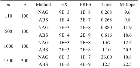
The testing was done on 4 families (A, B, C and D) of well-conditioned, ill conditioned, full rank, rank deficient and a few specific benchmark problems. The accuracy was specially obtained over NAG QR code [18] based upon QR factorization via Householder rotations. Hence due to the notable better computational performance, ABS algorithm with modified Huang method with LLS problem in [19] is found suitable for solving proposed problem. Table 1 shows the comparison of ABS algo- rithm with NAG code where EX stands for relative error in the solution, ERES stands for relative error in the residual, M-flops stands for Mega flops and m and n show

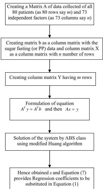
[image:3.595.308.541.621.735.2]

the number of rows and columns respectively [15]. These results are one of the examples of ABS algorithm efficiency in terms of time and accuracy. Figure 1 shows the flowchart of the steps followed for modeling the regression equation using ABS class of algorithms.

Table 1. Comparison of ABS vs NAG code for classical techniques for solving LLS.

m n Method EX ERES Time M-flops NAG 9E−3 1E−8 0.268 9.6 110 100

ABS 1E−4 3E−7 0.268 9.8 NAG 7E−3 2E−8 0.880 11.9 500 100

ABS 9E−4 2E−9 0.616 18.6 NAG 1E−3 2E−8 1.67 12.4 1000 100

ABS 2E−3 2E−8 1.10 20.5 NAG 6E−3 1E−7 26.00 10.8 1500 300

ABS 1E−3 4E−9 12.5 22.5

(4)

Creating matrix b as a column matrix with the sugar fasting (or PP) data and column matrix X

as a column matrix with n number of rows

Creating a Matrix A of data collected of all 80 patients (as 80 rows say m) and 73

independent factors (as 73 columns say n)

Creating column matrix Y having m rows

Formulation of equation

T T

A yA b and then Axy

Solution of the system by ABS class using modified Huang algorithm

Hence obtainedxand Equation (7) provides Regression coefficients to be

[image:4.595.67.276.79.462.2]

substituted in Equation (1)

Figure 1. Flowchart of implementation of ABS algorithm for detection of sugar fastening level and PP.

2.3. Data Surveyed

A Survey on 80 patients has been done at an Endocri- nologist’s (one of the author’s) patients for the number of factors affecting diabetes 73. All these 73 factors are taken as independent variables; sugar fasting and Post- Prandial (PP) sugar as dependent variables. The factors affecting diabetes include: Age; Height; Weight; BMI; Waist Circumference; Waist Hip ratio; Biceps; Triceps; Suprailiac; Sub scapular; Total lipids; Phospholipids; Triglycerides; Total Cholesterol; HDL; LDL; VLDL; HOMA-B; HOMA-R; Insulin; Hb1Ac; Hb1Ac (%); E:I Ratio; S:L Ratio; Pulse Rate; Fat in grams: L arm BMC; L arm Fat; L arm Lean; L arm Lean + BMC; L arm Total Mass; L arm % Fat; R arm BMC; R arm Fat; R arm Lean; R arm Lean + BMC; R arm Total Mass; R arm % Fat; Trunk BMC; Trunk Fat; Trunk Lean; Trunk Lean + BMC; Trunk Total Mass; Trunk % Fat; L Leg BMC; L Leg Fat; L Leg Lean; L Leg Lean + BMC; L Leg Total Mass; L Leg % Fat; R Leg BMC; R Leg Fat; R Leg Lean;

R Leg Lean + BMC; R Leg Total Mass; R Leg % Fat; Subtotal BMC; Subtotal Fat; Subtotal Lean; Subtotal Lean + BMC; Subtotal Total Mass; Subtotal % Fat; Head BMC; Head Fat; Head Lean; Head Lean + BMC; Head Total Mass; Head % Fat; Total BMC; Total Fat; Total Lean; Total Lean + BMC; Total Mass; Total % Fat.

3. Numerical Solution

An illustrative example of the solution of LLS through the ABS class of linear systems, which has been verified with the other methods on wikipedia [20] is described as follows:

1 2 6; 1 2 2 5; 1 3 2 7; 1 4 2 10

x x  x  x  x  x  x  x 

Comparison with Axb gives

1

1 2

2 3

4

1 1 6

1 2 5

, , ,

1 3 7

1 4 10

y

x y

A b x y

x y

y

 

   

 

    _{ }

 

   

  _{ } 

 

    _{ }

 

   

     

T 1 1 1 1 _,

1 2 3 4

A   _

 

1

2

T T

3

4

6

1 1 1 1 1 1 1 1 5

1 2 3 4 1 2 3 4 7

10 y

y A y A b

y

   

   

 _{ }  _{ }

 _ _ _ _

   

   

   

   

T 28 _so T 28

77 77

A b _{ } A y_{ }

   

0 0

Let 1 1

0 1 0 0 0

0 0 1 0

,

0 0 0 1

0 0 0 0 1

x H

   

   

  

  

   

   

k

k k

S H a ,

1 1 1

1 0 0 0 1 1

0 1 0 0 1 1

0 0 1 0 1 1

0 0 0 1 1 1

S H a

     

     

  

     

     

T

1 1

For 1

i i i

p H Z

i p H



  Z₁

1

1 0 0 0 1 1

0 1 0 0 1 1

0 0 1 0 1 1

0 0 0 1 1 1

p

     

     

 

     

     

Condition T ₀

i i i

(5)





1 0 0 0 1 0 1 0 0 1

1 1 1 1 4.

0 0 1 0 1 0 0 0 1 1

                        Hence satisfied, Now,





 

T 1 1 1

2 1 _T

1 1

a x b

1

x x P

a P  _         









2 0 1 1 1 1 0 28

0 1

0

0 1

0 1 1

1 1 1 1 1 1 x    _{ }           _{ }       _{ }_{ }                             _ _{ } _        _{ }   









T 1 1

2 2 1 _T

1 1 7 7 , 7 7 P P

x H H

P P               





T 1 1 1 1

, 1 1 1

1 1 P P               1









2 1 1

1 1 1 1

1 0 0 0 1

0 1 0 0 1

1 0 0 1 0

1 0 0 0 1

1 1 1 1 1 1 0.75 0.25 0.25 0.25 0.25 0.75 0.25 0.25 . 0.25 0.25 0.75 0.25 0.25 0.25 0.25 0.75 H                           _{ } _   _  _         _{ }  _{ }  _{ }  _{ }        _ _ _         _ _ _    Now, T

2 2 2

0.75 0.25 0.25 0.25 1 1.5 0.25 0.75 0.25 0.25 2 0.5 . 0.25 0.25 0.75 0.25 3 0.5 0.25 0.25 0.25 0.75 4 1.5 p H Z

      _ _ _           _ _ _    Now, T 2 2 2

3 2 T

2 2 a x b

2

x x p

a p     _{ } _  









3 7 7

1 2 3 4 77

7 7 1

7 7 0

1.5

7 0

0.5

7 1

1 2 3 4 0.5 1.5 x          _{  } 

    _ _.5

.5 .5 .5   _ _      _ __         _{ }_{ } _ _         _ _ _ _         _   _        _ _       3 4.9 6.3 . 7.7 9.1 x             

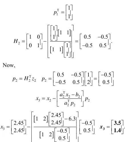
The above equation is obtained for ABS linear problem and applying it to finding solution of Linear Least Square Problem,

1

2

1 1 4.9

1 2 6.3

, ,

1 3 7.7

1 4 9.1

x

A b x

x         _{ }       _{  }     _{ }        

Let for the equation Axb

1 1

0 1

,

0 0

x H 0

1    _{ } _ _     k k k

S H a

1 1 1 1

1 0 1

,

0 1 1

S H a H _  _{ }

      i T i i

p H z

T 1 1 1

1 0 1 1

0 1 1 1

p H z _     _{    }

     

T 1 1 1

2 1 T

1 1 a x b

1

x x p

a p                _                 

 

2 0

1 1 4.9

0 0 1 2.45

1

0 1 2.45

1 1 1 x            _ _{ } _  _{ }_ __{ }        _ _            T 1 1

2 1 T

(6)

T 1

1 1

p    

 

 

2 1 1 1

1 0 1 0.5 0.5

. 1

0 1 0.5 0.5

1 1 1 H       _   _  _   _ __ __ _      _ _          Now, T 2 2

p H z₂ ₂ 0.5 0.5 1 0.5 0.5 0.5 2 0.5 p _     _{   } 



    

 

T 2 2 2

3 2 T

2 2 a x b

2

x x p

a p     _{ } _  









3 2.45

1 2 6.3

2.45

2.45 0.5

2.45 _{1 2} 0.5 0.5

0.5 x   _{ }      _   _   _ _ _ _             _ _    .  x3   _1.4

3.5 4 t t t t t t t

Hence, the solution has been verified with the other classical methods.

4. Results and Conclusion

Proposed work contains two aims: First to find out the regression equation relating all the factors affecting diabetes with the sugar fasting level and PP; Second is to find out the strength of relationship among sugar fasting level and PP with these factors, that is clear from the below mentioned Equations (A) and (B) by their weights in the equation. General available softwares for regression analysis do have their limits for the number of independent variables and the data size i.e. for Microsoft Ex-

cel it is limited to 16 variables, this is not a case for presented program. The programming has been done is C language. The Regression equations obtained are:

1 1 2 3

5 6 7 8 9

10 11 12 13 14

15 16 17 18 19

20 21

8.540 0.4103 1.8127 0.291 0.8983 1.2169 1.1023 0.298 0.6106 0.020 0.0699 0.0168 0.0401 0.04 0.0213

0.4012 0.06 0.172 1.4998 71.091

42.08 13.163

y t t t

t t t t t

t t

    

    

    

    

  ₂₂ ₂₃ ₂₄

25 26 27 28 29

30 31 32 33 34

35 36 37 38 39

40 41

0.8 3.016 4.9329

0.8919 0.2969 0.001 0.0051 0.0051

0.0017 0.1722 0.0168 0.0018 0.0086 0.0088 0.0041 0.1774 0.031 0.0002 0.002 0.0021 0.0006

t t t

t t t t

t t

  

    

    

    

   ₄₂ ₄₃ ₄₄

45 46 47 48 49

50 51 52 53 54

55 56 57 58 59

60 61 62

0.038 0.051 0.0008 0.0015 0.0009 0.0034 0.3142 0.0128 0.0021 0.0008 0.0002 0.0004

0.2034 0.002 0.0001 0.0002 0.0001

0 0.201 0.0129 0.000

t t t

t t t t

t t t t t

t t t t

t t t

 

    

    

    

    ₆₃ ₆₄

65 66 67 68 69

70 71 72 73

9 0.0019

0.0028 0.0036 0.616 0.0063 0

0.0002 0.0002 0.0001 0.0799

t t

t t t t t

t t t t



    

   

(A)

2 1 2 3 4

5 6 7 8 9 10

11 12 13 14 15 16

17 18 19 20

21 22

11.653 3.912 0 12.014 2.171 20.0103 6.4121 8.11 0 10.988 0 0.061 7.098 1.251 5.2113 5.002 0 0.5027 0.1831 90.0121 33.5166

161.1213 0 341.904

y t t t t

t t t t t t

t t t t t

t t t t

t t

    

     

     

   

   23 24 25

26 27 28 29 30 31

32 33 34 35 36

37 38 39 40 41

42 43 44 45 46 47 48 49

8 0 0.411

2.0051 0 0.089 0 0.019 0

291.113 0 291.76 291.531 0 1.0056 194.1214 0 193.535 193.314

0 0 0 0 0 0 0 0

0.9012

t t t

t t t t t t

t t t t t

t t t t

t t t t t t t t

t                          

 ₅₀ ₅₁ ₅₂ ₅₃ ₅₄ ₅₅

56 57 58 59 60 61 62

63 64 65 66 67 68 69

70 71 72 73

0 0.6655 0.6655 0.0052 0

0 0.0007 0 0 0 2.9648 0

0.0931 0.4101 0 0.201 0 0 0

0.0011 0 0 0

t t t t

t t t t t t t

t t t t t t

t t t t

                       t t t (B)

y1 and y2 present the sugar fasting and PP levels respec-

tively, whereas 1 2 3 73 are the independent vari-

ables in the same order as discussed in 2.3. However, merely the regression coefficients cannot conclude about the significance of relationship between the parameters. Since, the scope of proposed study is limited towards finding the regression equation via ABS algorithm, not the p values and the significant impact of independent variables on the dependent one. The weights in regression equation have been used for further discussion for the proposed study and are summarized in Table 2.

, , , , t t t  t

For sugar fasting level:

[image:6.595.62.281.79.327.2]

1) It can be observed that the regression coefficients of HOMA-R, Hb1Ac, E:I ratio, HOMA-B, height, waist circumference, pulse rate, BMI, insulin (negative value), S:L ratio (negative value) were the top 10 positive/negative parameters (largest regression coefficient values), showing their observable impact on sugar fasting (y1).

Table 2. Top 10 most influencing factors affecting sugar fasting and PP.

Parameters Regression coeff. for sugar fasting

Regression coeff. for PP

Height 1.8127 -

S:L ratio −4.9329 -

Pulse rate 0.8919 -

BMI 0.8983 - Waist circumference 1.2169 -

HOMA-B 1.4998 -

HOMA-R 71.091 90.0121

Insulin −42.08 −33.5166

Hb1Ac 13.163 161.1213

E:I ratio 3.016 −341.9048 R arm Fat - −291.76 R arm Lean - 291.531 R arm % fat - 194.1214

Trunk Fat - 193.535 Trunk Lean - -193.314

(7)

2) The regression coefficients of subtotal lean, subtotal lean + BMC, subtotal total mass, total fat, total mass have the smallest values; hence they are the parameters having least effect on either increase or decrease in sugar fasting level (y1).

For PP level:

1) It can be observed that the regression coefficients of biceps, weight, HOMA-R, Hb1Ac, trunk lean, trunk BMC, R arm lean + BMC, E:I Ratio (negative value), trunk lean + BMC (negative value), insulin (negative value) were the top 10 positive/negative parameters (largest regression coefficient values), showing their observable impact on PP (y2).

2) The regression coefficients of a large number of parameters have the small values depicting no impact on PP (y2).

Further development of the work could be in the direc- tion of application of LLS via ABS algorithm for more applications i.e. ANOVA and Chi-square, finding out the

coefficient of determination for the significance of strength of correlation, polynomial fitting, numerical smoothing & differentiation and modelling workhorse & process modelling. Besides more ABS algorithm variants can be used for LLS, linear programming and non-linear programming problems due to their vast applicability in real life problems. The binary diabetes parameters can be solved by logistic regression using integer programming applications of ABS algorithms.

5. Acknowledgements

We wish to thank the Executive Director, Birla Institute of Scientific Research for the support given during this work. We gratefully acknowledge financial support by BTIS-sub DIC (supported by DBT, Govt. of India) and Advanced Bioinformatics Centre (supported by Govt. of Rajasthan) at Birla Institute of Scientific Research for infrastructure facilities for carrying out this work.

REFERENCES

[1] E. Spedicato, E. Bodon, Z. Xia and N. Mahdavi-Amiri, “ABS Method for Continuous and Integer Linear Equa- tions and Optimization,” Central European Journal of Operations Research, Vol. 18, No. 1, 2010, pp. 73-95. doi:0.1007/s10100-009-0128-9

[2] S. Lalwani, R. Kumar, E. Spedicato and N. Gupta, “An Application of the ABS LX Algorithm to Multiple Se- quence Alignment,” Iranian Journal of Operations Re- search, Vol. 3, 2012, pp. 31-45.

[3] S. Lalwani, R. Kumar, V. Rastogi and E. Spedicato, “An Application of the ABS LX Algorithm to Schedule Me- dical Residents,” Journal of Computer and Information Technology, Vol. 1, 2011, pp. 95-118.

[4] S. S. Rich, “Genetics of Diabetes and Its Complications,” Journal of the American Society of Nephrology, Vol. 17, No. 2, 2006, pp, 353-360. doi:0.1681/ASN.2005070770 [5] World Health Statistics Report, 2012.

http://www.diabetes24-7.com/?p=1272

[6] A. Ramachandran, C. Snehalatha, A. S. Shetty and A. Nanditha, “Trends in Prevalence of Diabetes in Asian Countries,” World Journal of Diabetes, Vol. 3, No. 6, 2012, 110-117. doi:0.4239/wjd.v3.i6.110

[7] C. L. Lawson and R. J. Hanson, “Solving Least Squares Problems,” Society for Industrial and Applied Mathemat- ics, 1995. doi:0.1137/1.9781611971217

[8] A. Bjõrck, “Numerical Methods for Least Squares Prob- lems,” Society for Industrial and Applied Mathematics, 1996. doi:0.1137/1.9781611971484

[9] J. Abaffy, C. G. Broyden and E. Spedicato, “A Class of Direct Methods for Linear Equations,” Numerische Ma- thematic, Vol. 45, 1984, pp. 361-376.

[10] J. Abaffy and E. Spedicato, “Numerical Experiments with the Symmetric Algorithm in the ABS Class for Linear Systems,” Optimization, Vol. 18, No. 2, 1987, pp. 197- 212. doi:0.1080/02331938708843232

[11] J. O. Rawlings, S. G. Pantula and D. A. Dickey, “Applied Regression Analysis: A Research Tool,” 2nd Edition, Springer, Berlin, 1998. doi:0.1007/b98890

[12] S. Chatterjee and A. A. S. Hadi, “Regression Analysis by Example,” 4th Edition, Wiley Interscience, 2006. doi:0.1002/0470055464

[13] H. Y. Huang, “A Direct Method for the General Solution of a System of Linear Equations,” Optimization Theory and Application, Vol. 16, No. 5, 1975, pp. 429-445. [14] E. Spedicato and E. Bodon, “ABSPACK 1: A Package of

ABS Algorithms for Solving Linear Determined, Under- determined and Overdetermined Systems.”

www.unibg.it/dati/persone/636/404.pdf

[15] E. Spedicato, “ABS Algorithm for Linear Systems and Linear Least Squares: Theoretical Results and Computa- tional Performance,” Scientia Iranica, Vol. 1, 1995, pp. 289-303.

[16] J. Abaffy and E. Spedicato, “ABS Projection Algorithms: Mathematical Techniques for Linear and Nonlinear Equa- tions,” Ellis Horwood Ltd., Chichester, 1989.

[17] E. Spedicato and E. Bodon, “Solution of Linear Least Squares via the ABS Algorithms,” Mathematical Pro- gramming, Vol. 58, No. 1-3, 1993, pp. 111-136.

doi:0.1007/BF01581261

[18] Numerical Algorithms Group (NAG) Codes. http://www.nag.co.uk/

[19] E. Spedicato, “On the Solution of Linear Least Squares through the ABS Class for Linear Systems,” AIRO Con- ference, 1985, pp. 89-98.

[20] Linear Least Squares (Mathematics), Motivational Exam- ple on Wikipedia.