Ray Tracing using 3D Grid Simulations
Ryan Thomas and Sudhanshu Kumar Semwal
Abstract—Bounding Volume Hierarchies (BVHs) and k-d trees have been used to create interactive ray tracing. Ray tracing dynamic scenes using nVidia’sR
OptiXTM has already provided thirty to sixty frames per second or better. In this paper, we implement space partitioning methods, such as grid method and the proximity clouds (PCs), on multiple GPUs. Our motivation is to investigate the use of such methods for medical applications, because there is direct one to one correspondence between 3D voxels used in space partitioning methods and 3D voxels in the volume data. In the past, proximity Clouds have worked well on static scenes, but object movement forces recalculation of the scene and some preprocessing cost. This paper investigates parallelizing these techniques on the GPU to determine the feasibility of dynamic scenes using them. Our scenes are made of spheres instead of volume data because at this time we do not know of any technique that can generate dynamically changing volume data. Interestingly, Proximity Clouds (PCs), which typically has large gains in rendering times compared to the 3D Grid method, emerges only slightly better than the 3D Grid method for dynamic scenes because both the processing and rendering costs are now added for dynamic scenes with spheres. The 3D grid method, due to its simpler preprocessing, may be the best choice for ray tracing the dynamic volume data on multiple GPU.
Keywords:3D Graphics, Ray Tracing, 3D Grids, CUDA. I. INTRODUCTION
T
HE goal of any grid structure is to divide the scene into voxels. These voxels are populated with the objects in the scene, and allow the ray to test only objects in the voxel intersected by the ray. The 3DDDA method [9] removes many unnecessary collision detection tests in favor of grid traversal. The Proximity Clouds(PC) method [3] builds from 3DDDA. PCs allow for a ray to skip a larger portion of the grid by computing how far the ray can safely jump before it might have a collision.Cellular automata (CA) [29], [22] could implement multi-level interactions, and emergence of diseases [26], [2]. Complex Systems science [12] has been applied to model events occurring in nature. Works by Prigogine [16], in thermodynamics, and earlier work by Poincare’s on sensi-tivity of dynamical systems to initial conditions provide the basis for complex systems research for cellular automata research. Limitations of simulating organic life by using computational models have been discussed before, these include (i) brittleness [18] of the computational medium, and (ii) the limitations of reductionist approaches to model organic life, which is well documented in [19]. Because Cellular Automata uses local interactions, not the reductionist approaches, it could provide a suitable platform to model organic behavior such as cancerous growth patterns. Local interactions, usually implemented for every cell, could create
Manuscript received July 5, 2014; revised July 30, 2014.
Ryan Thomas and Sudhanshu Kumar Semwal are with the Department of Computer Science, University of Colorado at Colorado Springs, CO, 80918, USA e-mail: [email protected] and [email protected]
subtle interactions mimicking organic behavior. Many exam-ples, such as flocking, and 3D games have shown remarkable variety of emergence when a cell’s next state is based on consulting nearby voxels. For example twenty-seven cells could be consulted for (3x3x3= 27; 26 immediate vicinity, and 1 itself) to decide the next state. Different non-linear and dynamics pattern could emerge using different local interactions strategies [17].
Volume Data provides one-to-one correspondence for use by a Cellular Automata. The Visible Human Project sup-ported (1989-2000) by US National Library of Medicine (NLM) provides a detailed volume data of human body. The process created a very detailed database of volume data 1 mm apart for the male cadaver with 1871 slices, which when stacked create a 3D grid of volume. This created 40 Gigabyte of 3D grid data which might have to be ray traced, or variation of raytracing called ray-casting could be used. 3D Morphing techniques [20], and for medical applications [7], [8] have been implemented using cellular automata on volume data. However, real-time manipulation of such large data is not possible with the computer systems of today, yet GPU computing provides a promising research direction. The rise of GPU computing has been growing over the previous few years. GPU computing allows for parrellization of algorithms when the algorithm allows for it. The 3DDDA traversal algorithm remains the same when run on the GPU and the CPU. Proximity Clouds are allowed a different approach on the GPU. The traditional algorithms proposed can be mapped on the GPU. The principles of the algorithm are the same but now are rewritten using a parallel processing implementation. The benefit is the loop is simplified allowing the distance calculations to be run simultaneously while building the Proximity Clouds. These adjustments make 3DDDA/Proximity Clouds the best choice on today’s hardware for dynamic scenes.
II. OCT TREES AND 3DDDA
Fig. 1. City Block Distance.
The size of the grid does matter as well. There is a tradeoff between memory and speedup. The smaller the voxels the fewer the objects a ray will have to test against. If a scene is represented by four voxels then it is still possible that lot of unnecessary collision calculations would have to be computed, but the memory footprint of voxels would be small. If the grid represents a single 1x1x1 unit in space, then number of collision would reduce but there would be a larger memory footprint. At some point, however, reducing the size of grid, may force the ray to traverse empty voxels which could be avoided if the voxels were larger. This observation is the basis for the Proximity Cloud method.
A. Proximity Clouds
In 1994 Cohen and Sheffer[3] proposed another grid traversal technique to speed up the ray tracing algorithm. Similar to the 3DDDA method, the scene is divided into many voxels. Once divided the grid cells determine a safe distance a ray may skip between voxels. This results in faster traversal of the voxel grid. When a ray hits a voxel, it first determines if any objects need to be tested. If the voxel is empty or the ray did not intersect with any object, the ray skips ahead by the value the voxel says is safe to skip. This allows for fewer calculations when traversing the grid. There are a few ways this can be accomplished. Using distance transforms, these safe values are calculated during preprocessing.
A method that determines a safe distance to skip is the minimum Euclidian distance between a voxel and all of the non-empty voxels. This would give the most accurate reading for a safe distance. A more optimized method is the city block distance method.
The city block distance is calculated by taking the differ-ence in x, y, and z of the current voxel with a non-empty voxel and summing it. This is performed for all of the voxels in the grid. This is not as accurate as the Euclidian distance, but it lets the program avoid calling the square root function on each of the cells. In order to compensate for the possibility of overshooting the target, the ray is normally brought back a grid cell, which ensures that no objects are missed, and then allowed to continue. In the worst case for Proximity Clouds when for the ray moves to the next cell, Proximity Cloud method become the 3DDDA method. This technique works great when a scene is divided across large areas, but for very close groups the cost of building the cloud may not justify the traditional 3DDDA method.
B. GPU Computing
Graphical Processing Units have become common in most computers today. They have been around since the 1980s with the goal of creating a rendering process for the system. This allows for better processing by freeing up the CPU from rendering by having dedicated hardware draw to the screens. GPUs are built with many processing cores that run in parallel. The trend has been that the GPU manufacturers are providing APIs for traditional processing on the GPU rather than just graphics rendering. Object hierarchy methods such as k-d tress [13] and BVHs [11] are used for these implementations. But the above mentioned approaches are based on partitioning the object space and may not be suitable for ray tracing 3D volume data as volume data does not have any objects to build the object hierarchies on.
One main advantage to using GPUs to run processing tasks is to give programmers access to more threading resources. Modern day CPUs generally have two to four cores on the standard desktops and up to sixteen cores on server CPUs. A device running on the GPU has the potential to have thirty-two threads on a single core. Threading is also made easier in languages such as CUDA. On the CPU it is up to the programmer to handle context switches during execution, but the GPU will begin working as soon as it is ready. This provides a massive amount of computing power in the average consumer computer. There are three main libraries out there that allow processing on the GPU: Microsoft’s DirectCompute (which is bundled with DirectX 11), OpenCL, and Nvidia’s CUDA library. We have used CUDA for our implementation.
The disadvantage is the memory constraints. For a GPU implementation we are limited to the memory free on the device. This is copied from the host(cpu) memory space, but this operation can be time consuming. This paper does not investagate acceleration techniques to buffer memory between the two, but it is a future topic to invesagate.
C. CUDA
CUDA runs exclusively on NVidia’s GPUs [13], [21]. It can be used as an extension to C or on its own. CUDA files traditionally consist of some host functions; functions run on the CPU and device functions, which run on the GPU. Communication between the host functions and device functions takes place through kernel methods. Host functions do not have the ability to directly call device functions. This function is accessible from a host and will run in multiple threads. A kernel function is called from the host in a different way.
III. IMPLEMENTATION
A. 3DDDA
The 3DDDA method on the GPU is similar to the version on the CPU. A grid is still built in a similar manner. The GPU implementation has the same algorithm when traversing the grid. It does fire many concurrent rays similar to the traditional one. The threads then traverse the global grid. The pre-processing is done in one kernel, and the traversing is done in another.
The first step is to determine which voxels are filled and which are not. The grid is a set size on the GPU since dynamic allocating and releasing of memory prevents real time rendering. Each voxel is made up of a structure. Each voxel contains a boolean to determine if it contains any spheres, an array of indices for the spheres located in the voxel, and three integers describing the x, y, and z position. This helps in the parallelization since the voxel array is declared as a single dimension array.
Building the grid is done with two separate kernels. The first kernel is designed to empty the grid. This is needed to register spheres with the correct grid cell. This is threaded in the x and y directions. Each thread loops over the z direction setting each cell to empty and resetting the array value to -1, which represents the end of the list of spheres contained in the voxel. This array is static because the GPU prefers static memory to dynamic. This can become a limitation of the system; however, when looking at enough spheres to fill a single voxel other memory issues may be introduced. In that case a new grid of a different size can be built or that array can be increased. On certain cards the memory limitations may be met building the grid and should be taken into account.
Once the grid is reset, it needs to be populated with the spheres contained in the spheres array defined using a float3 data type. The float3 data type is defined in CUDA and contains three floats. The min and max of the sphere is determined in order to create a bounding box used to fill the voxels. Spheres also define a material, which determines their reflectiveness and color. An array on the GPU defines the spheres that are to be rendered. This global array is used to populate the voxels in a second kernel. This kernel is a single dimensional kernel that threads on the number of spheres. Each sphere fills the cells that are contained within its bounding box. Once this kernel is finished the grid traversal can begin.
The final kernel in the process draws the scene. It is broken up in the same way as traditional ray tracing, but it does not compute the collision for each sphere, rather traversing the grid in a device function.
B. GPU Proximity Clouds
Proximity Clouds was built using a variety of distance computations. All of them require at least an n squared al-gorithm to compute, usually two pass alal-gorithm as described in[3] is implemented. These algorithms can be parallelized to run on the GPU. The algorithm presented in this paper is as follow. The index represents the voxel that needs to determine its distance. The thread in the y direction represents a voxel that is not empty. If a thread receives a voxel that is empty, the thread returns and asks for the next voxel. Once all threads in a block are completed a new block
is loaded on the GPU. This builds the clouds in a way that can be scaled to multiple GPUs and can run on any GPU. It is possible to run this in a single warp when sufficient threads are available. This algorithm can take any distance computation to determine a safe distance to jump.
The speed of this algorithm comes from the parallelization of the system. The first list is divided up into many different threads so they can run in sync. The PC generated for the experiment consisted of a 40x40x40 grid. The list is 64,000 in length and the second list would be of equal size for the worst case.
IV. RESULTS
The results were run on a Windows 7 64 bit PC with 6GB of RAM, an Intel i7 2.66 GHz processor, and an NVidia GTX 570 graphics card. The GTX 570 has 480 CUDA cores with a graphics clock of 732 MHz and a processor clock of 1464 MHz.
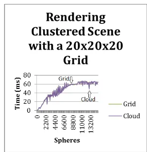
[image:3.595.350.498.317.470.2]A. Clustered Spheres Performance
Fig. 2. Clusted preformance of the grid and cloud
The first result looks at rendering up to 15,000 spheres in a scene using a 20 by 20 by 20 grid. This grid size was chosen because larger ones would time out when building as discussed later. Since the scene has no real gaps it is expected that the cloud and the grid would perform at the same speed. The proximity cloud only produced a .3% increase in speed, but it did speed up traditional ray tracing by 91.8%. One item to take note of is the bouncing of the line. When testing, spheres are generated at positions in the scene by looping in the x and y directions, trying to reduce the difference of x and y creating a balanced scene. The goal was to create large and evenly spaced scene. There are cases where more spheres wind up outside of primary rays causing a faster result.
B. Clustered Spheres with Large Grid
To better demonstrate the performance of a larger grid, the same scene as above was generated using a 40x40x40 grid. Far fewer spheres are used due to the timeout that can occur when building the Proximity Clouds with the addition of rendering.
Fig. 3. Clustered preformance including non optimized ray tracer
Fig. 4. Clusted preformance of the grid and cloud
are no large empty areas. There is a 6% increase in speed when looking at proximity clouds over the grid method, and a 79% increase in speed over traditional ray tracing.
C. Rendering Planes of Spheres
In order to showcase the advantage that has been claimed for Proximity Clouds, a new scene was generated, where two planes of spheres are created. One plane is toward the front of the scene, while the second plane is far at the back. This allows for a large gap between them demonstrating how Proximity Clouds increases rendering time. The grid and Proximity Cloud methods show much faster performance over non optimized ray tracing. The difference between proximity clouds and the 3DDDA method is not as large as expected. This is partially due to the size of the grid. A 40x40x40 grid can only skip the length of the grid in the best case. This does not allow for huge performance increases when each thread is traversing the grid simultaneously. The average increase in speed was only 6.4% when looking at all points on the graph, but a 94.2% increase from the non-optimized ray tracer was achieved. As the scene grows and becomes sparser this should only increase.
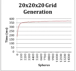
D. Proximity Cloud Generation Speed
[image:4.595.344.499.107.343.2]The next set of data that needs to be looked at is the speed at which proximity clouds can be generated. This is based on the size of the proximity cloud, as well as how populated the scene is. Each test below generates spheres in random locations and tests the speed at which the Proximity Clouds can be generated.
[image:4.595.98.243.225.358.2]Fig. 5. Sparsly populated grid
Fig. 6. 10x10x10 grid generation
[image:4.595.353.500.439.575.2]When building a 10x10x10 grid, it can be put in a single warp. Building it only takes 1ms, which is a single loop through the scene.
Fig. 7. 20x20x20 grid generation
A 20x20x20 cloud is a little bigger, but it experiences a similar behavior to the 10x10x10 cloud. Once at 350ms it begins to level out no matter the number of spheres added because the scene has a sphere in every voxel.
While slower the 30x30x30 grid is still manageable. Similar to the 20x20x20 grid, the 30x30x30 builds in the same time scale. This is due to a large number of CUDA cores working in parallel. The 30x30x30 grid requires the same number of warps as the 20x20x20, thus completing in the same amount of time.
Fig. 8. 30x30x30 grid generation
Fig. 9. 40x40x40 grid generation
speed of Proximity Clouds so that its closer to the speed it takes to build the 10x10x10 grid. Still the speed to build the Proximity Clouds plus the time to render is still faster than the traditional ray tracer. It is not necessarily faster than the grid method, but it is only slightly better.
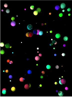
[image:5.595.94.243.137.287.2]There were no differences when between the rendering techniques. The image below is an example of a rendering.
Fig. 10. Ray Tracing large number of spheres.
V. OBSERVATIONS
The work presented here shows massive speedups to the overall rendering of the scene. The baseline between a traditional ray tracer in C and the code running in CUDA clearly shows the advantage of using a GPU. This result shows the amount of parallelization that a ray tracer contains. By allowing each primary ray its own thread on a GPU, the system was able to run in fraction of the time. The GPU version does have limitations compared to its CPU counterpart. A CPU does theoretically have infinite time to
render the scene. The tests conducted here were required to finish in five seconds on an NVidia GTX series GPU. The CPU is also only limited by the system RAM or 4GB on a 64-bit machine, which is generally much larger than the GPU. The 3DDDA method on the GPU offers a huge speedup over the traditional method on the GPU. Scenes containing over ten thousand spheres would render in seconds with the traditional method, but milliseconds with the grid. This is due to limiting the number of collision detection operations on a per thread basis. Memory did limit the maximum grid size in the experiments. The grid used was 40x40x40, which resulted in 64,000 voxels. This is due to a limitation in CUDA only allowing the indexing of 216 continuous array cells. This still greatly increased the speed, but smaller more accurate grids can also provide much faster results. The smaller the grid the fewer collisions take place, making it important to maximize the grid size.
The speedup between the 3DDDA method and the tra-ditional method was expected. The Proximity Clouds did not add as drastic of a change. This is due to the size of the clouds and the way a GPU works. It is possible several rays finished faster using the GPU method, but they all must finish for a new warp to start. The proximity clouds may speed up individual rays but not a cluster of them in a GPU warp.During rendering the Proximity Clouds were faster than the 3DDDA method. That speedup was very useful, but building of the clouds forced the speed to come closer to the original method. This still was able to render many more spheres than the original. The clouds were built in one kernel, and the rendering was done in another. This would allow for a maximum of 10 seconds of total processing time before a GPU would time out for the entire computations. Similar to 3DDDA the rendering is limited to memory before it hits the timeout.
The speed of the Proximity Clouds method can increase if multiple GPUs are used to build them or preprocessing time could be counter separately not in the rendering. It also can be buffered ahead. While rendering a second GPU can be used to build the clouds for the next scene.
VI. CONCLUSIONS
[image:5.595.97.241.428.623.2]better capability to handle large voume data sets to ray trace voume data sets in real-time, and to implement cellular automata based algorithms for medical applications. The speed increase between the clouds and 3DDDA on the GPU demonstrates that more work should be done to come up with better traversal methods, and continued parallelization of both preprocessing and rendering algorithms will only result in a better speedup.
REFERENCES
[1] Appel, Arthur. ”Some Techniques for Shading Machine Render-ings of Solids.” ACM Digital Library. Web. 03 Apr. 2011. http://portal.acm.org/citation.cfm id=1468082.
[2] Bezzi M, Modeling Evolution and Immune System by Cellular Au-tomata, http://citeseer.nj.nec.com/429312.html
[3] Cohen, Daniel, and Zvi Sheffer. ”Proximity Clouds an Acceleration Technique for 3D Grid Traversal.” The Visual Computer 11.1 (1994): 27-38.
[4] Daniel CohenOr, Amira Solomovic, David Levin, Three-Dimensional Distance Field Metamorphosis, ACM Transactions on Graphics (TOG), Volume 17,Issue 2, Pages:116-141, 1998.
[5] Dauenhauer, David, and Sudhanshu K. Semwal. ”Approximate Ray Tracing.” Graphics Interface (1990): 75-82. Print.
[6] ”Download Details: DirectX 11 DirectCompute: A Teraflop for Every-one.” DirectX 11. Microsoft. Web. 3 Apr. 2011.
[7] S. Fang and R. Raghavan and J. Richtsmeier, Volume Morphing Meth-ods for Landmark Based 3D Image Deformation, SPIE International Symposium on Medical Imaging: 1996
[8] Tom Forsyth, Cellular Automata for Physical Modeling, Game Pro-gramming Gems 3: pp. 200-214, 2002.
[9] Fujimoto, Akira, Takayuki Tanaka, and Kansei Iwata. ”ARTS: Acceler-ated Ray-Tracing System.” IEEE Computer Graphics and Applications 6.4 (1986): 16-26. Print.
[10] Glassner, Andrew S. An Introduction to Ray Tracing. London: Aca-demic, 1989. Print.
[11] Dinesh Manocha and Christian Lauterbach. ”Ray Tracing Dynamic Scence using BVHs,” SigGraph 2006 presentation, pp. 1-47 (2006). [12] Melaine Mitchell, Complexity: A Guided Tour, pp.1-337, Oxford
University Press 2009.
[13] ”NVIDIA CUDA C Programming Best Practices Guide.” CUDA Programming Guide. NVIDIA, July 2009. Web. 10 Mar. 2011. [14] ”OpenCL.” The Khronos Group: Open Standards, Royalty
Free, Dynamic Media Technologies. Web. 03 Apr. 2011. http://www.khronos.org/opencl/.
[15] NVidea – OptiX(TM) Ray Tracing Enginge. ”Programming Guide,” OptiX Programming Guide.pdf, pp. 1-71 (2008).
[16] Prigogine, I. From Being to Becoming, Freeman ISBN 0-7167-1107-9. [17] Rabinovich MI, AB Ezesky, PD Weidman, The Dynamics of Patterns,
pp. 1-324, World Scientific (2000).
[18] Thomas Ray, An Evolutionary Approach to Synthetic Biology: Zen and the Art of Creating Life, Chapter 2, Book on best papers from VW98 Paris Confeerence (2000).
[19] Stephen Rothman, Lessons from the Living Cell: The Limits of Reductionism, McGraw Hill, pp. 1-300.
[20] SK Semwal and K Chandrashekher, 3D Morphing for Volume Data, pp 1-7, The 18th conference in Central Europe, on Computer Graphics, Visualization, and Computer Vision, WSCG 2005 Conference, January 2005.
[21] Sanders, Jason, Edward Kandrot, and J. J. Dongarra. CUDA by Example. Upper Saddle River (N.J.): Addison-Wesley, 2011. [22] Palash Sarkar, A brief history of cellular automata, ACM Computing
Surveys (CSUR) Volume 32 , Issue 1, pages 80-1-7, 2000.
[23] Semwal, Sudhanshu K., and Hakan Kvanstrom. ”Directed Safe Zones and the Dual Extent Algorithms for Efficient Grid Traversal during Ray Tracing.” Graphics Interface (1997): 76-87. Print.
[24] Semwal, Sudhanshu K., Charulata K. Kearney, and J. Michael Moshell. ”The Slicing Extent Technique for Ray Tracing: Isolating Sparse and Dense Areas.” Graphics, Design and Visualization (1993): 115-22. Print. [25] Semwal, Sudhanshu K. ”The Slicing Extent Technique for Fast Ray
Tracing.” Computer Graphics 2.2 (1988): 88-89. Print.
[26] R. Sosic and Robert R. Johnson. Computational properties of self-reproducing growing automata BioSystems, 36:7-17, 1995.
[27] Suffern, Kevin G. Ray Tracing from the Ground up. Wellesley, MA: K Peters, 2007. Print.
[28] Whitted, Turner. ”An Improved Illumination Model for Shaded Dis-play.” ACM SIGGRAPH Computer Graphics 13.2 (1979).