Abstract— In engineering studies, normally the behavioral function of a system is, normally replaced by a number of measured values per known inputs – in the form of a table function. Sometimes it is necessary to access a system function in order to be able to study behavior of the system. This is where we normally approximate with a polynomial through a table function which is due to the special features of polynomial expressions. Different methods are used to approximate the behavior of a system with a polynomial expression including Lagrange and Newton interpolating polynomial expressions. Although Lagrange and Newton interpolations are meant for calculation per a given point, neither of them provide interpolating polynomials directly, and the coefficients are produced from combination of multiplication of several expressions. Reconsidering the relations in this study, we offer an algorithm for direct calculation of coefficients of different powers of x in an interpolating polynomial.
Index Terms— Neutral Points, coefficients of Interpolating, Lagrange Interpolation
I. INTRODUCTION
HE interpolation formula was discovered and introduced by Waring in 1779 and Lagrange interpolation was presented in 1795 [1]. The main Lagrange form has certain shortcomings, e.g., increasing the degree of the polynomial by adding a new interpolation point requires computations from scratch, and also the computation is numerically unstable [2]. Berrut et al. have modified Lagrange form and the barycentric Lagrange were introduced as a fast and stable method [3], overcoming the shortcomings of the original form and makes Lagrange interpolation suitable for practical application [2]. Many articles for efficient Lagrange interpolation algorithms are also published. Werner et al., showed that the Lagrangian form of the interpolating polynomial may be calculated with the same number of arithmetic operations as the Newtonian form [4]. Feng et al. studied how to obtain exact interpolation polynomial with rational coefficients by
Manuscript received March 03,14, 2015; revised April 04,9, 2015. S. R. Moasheri is with Education Organization of Razavi Khorasan, Education Ministry, Mashhad, Iran (e-mail: [email protected]).
A. Momeni is with the department of electrical and electronics, Shiraz university of technology, Shiraz 13876-71557, Iran (e-mail: [email protected]).
S. M. Moasheri is with Research Institute of Food Science and Technology (RIFST), Department of Food Biotechnology, Mashhad, Iran (e-mail: [email protected])
approximate interpolating methods [5]. Solares et al. have also explored the interpolation mechanism of the separable functional networks, when the neuron functions are approximated by Lagrange polynomials. The coefficients of the Lagrange interpolation formula were estimated during the learning of the functional network by simply solving a linear system of equations [6]. Some articles may compute the coefficients of interpolation, as Gonnet et al. considered methods to compute the coefficients of interpolants relative to a basis of polynomials satisfying a three-term recurrence relation [7].
The interpolation polynomial in most of studies, is produced from combination of multiplication of several expressions. It seems that calculation of coefficients is complex. In this paper, by rewriting the base form of Lagrange interpolation, we suggest the method to compute the direct and simple interpolation coefficients.
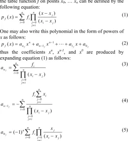
According to [3], Lagrange Interpolating Polynomial for the table function f on points x0, … xn can be defined by the
following equation:
0 0
( )
( )
( )
n n jf i
i j i j
j i
x x p x f
x x
(1)
One may also write this polynomial in the form of powers of x as follows:
1
1 1 0
( )
f f f f
n n
f n n
p x a x a x a x a (2)
thus the coefficients xn, xn-1, and x0 are produced by expanding equation (1) as follows:
0 0
( )
f
n
i
n n
i
i j
j j i
f a
x x
(3)
0 1
0 0
( )
f
n
i i
j n
j i
n n
i
i j
j j i
f x a
x x
(4)
0
0 0
( 1)
( )
f
n n
j n
i
i j i j
j i
x
a f
x x
(5)
It can be seen that calculation of coefficients of f
k
a
gets more complex as k approaches the 0 to n field.It seems due to the lack of a fixed relationship between the coefficients it is not possible to get iterative-based flowcharts for calculation of the coefficients for different values of n. Yet given equation (3) it is always easy to find the coefficient of the highest power of x. This study uses
Developing Two Novel Lagrange-based
Algorithms for Direct Calculation of
Interpolating Polynomial Coefficients
Seyed Reza Moasheri, Ali Momeni, Seyed Majid Moasheri
[image:1.595.305.557.419.696.2]equation (3) to calculate coefficient f
n
a
, and then applies a set of operations on the table function f, based on the proposed methods in such a way that 1f
n
a
can be recalculated from equation (3) (the same goes for other coefficients). As all coefficients are always calculated from the same equations it is possible to make an algorithm for it. Yet before proceeding to such methods we have first to prove a few theorems:II. NEW THEOREMS A. Theorem 1 (Retrieval)
If g(x) is a polynomial function of power n, any given n+1 point set of this function may be produced through interpolation.
Proof.
We assume a given n+1 point set of function g(x) in which xis are different two by two. We suppose that the function pg(x) is the result of interpolating per these same points.
Since pg(x) is produced by interpolating points, maximum
power of this function is n. Assuming that the power of pg(x) is l and less that n we have:
1
1 1 0
( )
g g g g
n n
n n
g x k x k x k x k (6)
1
1 1 0
( )
g g g g
l l
g l l
p x a x a x a x a (7)
Thus the function T(x) is defined as follows:
( ) ( ) g( )
T x g x p x (8)
Since pg(x) is produced by interpolation of n+1 points, it
coincides with g(x) at point n+1. Therefore, function T(x) must have at least n+1 roots. This is while function T(x) has at most n roots (because its power is n). Hence the assumption that the power of the interpolating polynomial pg(x) is lower than g(x) is not true.
But is the power of the interpolating polynomial pg(x)
equals that of function g(x) then we have:
1
1 1 0
( )
g g g g
n n
g n n
p x a x a x a x a (9)
In case since function pg(x) is produced from
interpolating n+1 points of function g(x), it coincides with g(x) at n+1 points, thus function T(x) must have at least n+1 roots. Since function pg(x) and g(x) are of the same power
the function T(x) may rewritten as follows:
1
1 1
1 1 0 0
( ) ( ) ( )
( ) ( )
g g g g
g g g g
n n
n n n n
T x k a x k a x k a x k a
(10) Thus the only way function T(x) can have at least n+1 roots is that
g g
i i
k
a
, in other words the result of interpolation equals the function itself.B. Theorem 2 (Mediating Polynomial)
It is always possible to add the polynomial function g(x) (with maximum power of n) per xis to the table function
f to calculate the interpolating function pf(x), and after
interpolation of the table function f+g subtract the function g(x) from the interpolating function pf+g(x) to get to the
interpolating function pf(x).
Proof.
Assuming table function f as:
x
x
0...
...
x
n
f
f
0...
...
i
f
Pf(x) would be;
0 0
( )
( )
( )
n n jf i
i j i j
j i
x x p x f
x x
(11)
If a polynomial function of maximum power n such as g(x) is added to function f per xis we will have the table
function as:
n
x
x
0...
...
i
x
)
(
...
...
)
(
00
g
x
f
ng
x
nf
i i
g
f
Now by interpolation we have:
0 0
( )
( ) ( ( ))
( )
n
n jf g i i
i j i j
j i
x x p x f g x
x x
(12)
thus,
0 0 0 0
( ) ( )
( ) ( )
( ) ( )
n
n
n
nj j
f g i i
i j i j i j i j
j i j i
x x x x p x f g x
x x x x
(13)
( ) ( ) ( )
f g f g
p x p x p x (14)
On the other hand we have:
( ) ( )
g
p x g x (15)
Because if we show the values of g(xi) with gi
n
x
x
0...
...
i
x
n
g
g
0...
...
i
g
There is always a unique polynomial function of maximum power n that includes all points of the table function g. Also since pg(x) is produced from interpolation
of n+1 points of nth power function g(x), according to Theorem 1 (Retrieval) the pg(x) will surely be the same
polynomial function g(x). Thus we have:
( ) ( ) ( )
f f g
p x p x g x (16)
Based on our discussion so far we can offer two methods for calculation of coefficients in interpolating polynomial expression: we know that the Lagrange interpolating polynomial is calculated by the table function f based on equation (1). It is obvious that maximum power of pf(x) is n.
As mentioned before, an may always be calculated from
equation (3). Now if we assume that pf(x) is of n-1 power,
then f
n
a
produced by equation (3) will surely be zero (in other words for n+1 points the pf(x) function is of n-1power) and to calculate 1 f
n
a
we must use equation (4). However, there may be other solutions as well.III. GENERATED NOVEL METHODS A. The first method
Assume that pf(x) is of the power of n-1 and is the result
interpolation of n+1 point. If we define:
( ) . f( )
g x x p x (17)
As function pf(x) is of power n-1 the pg(x) (is a result of
interpolation of xi.pf(xi)) is definitely of power n. Thus
( )
g
p x
( )
f
according to Theorem 1 (Retrieval) with any given set of n+1 points of function x.pf(x) we can produce the function
pg(x) from interpolation. Now if this n+1 point set is taken
as x0, … xn since xi.pf(xi)=xifi we can take the polynomial
function pg(x) as the interpolated form of the table function
gi=xifi. Thus pg(x) becomes:
1 2
1 0 1 1 0
( )
g g g f f f
n n
g n n
p x a x a x a a x a x a x(18)
When assuming that function pf(x) is of power n-1 then
g
n
a
will never be zero and equation (3) may be used for calculations.Assume that the table function f is as follows: n
x
x
0...
...
i
x
n
f
f
0...
...
i
f
Hence gi=xifi becomes0
...
nx
x
i
x
0 0
... x
n nx f
f
i i i
g
x f
Now, from equation (3) we have
0 0
1
g
n n
n i i
i j i j
j i
a f x
x x
(19)On the other hand we know that pf(x) is of power n-1 so
according to equation (4):
0 1
0 0 f
n
i j
j n
j i
n n
i
i j
j j i
f x a
x x
(20)
We can rewrite the equation (20) as;
0 1
0
0
0 0
0
( )
( )
f
n
i j i i i i
j n
j i
n n
i
i j
j j i
n
i j i i
n j n i
i j
j j i
f x f x f x a
x x f x f x
x x
0 1
0 0
0 0
( ) ( )
f
n
i j
n n
j i i
n n n
i i
i j i j
j j
j i j i
f x
f x a
x x x x
(21)
As 0 n
j j
x
is independent of i it may be taken out of thei
.1
0 0 0
0 0
( )
( ) ( )
f
n n n
i i i
n j n n
j i i
i j i j
j j
j i j i
f f x
a x
x x x x
(22)
so,
1
0 0
0
( )
( )
f f
n n
i i
n j n n
j i
i j
j j i
f x a x a
x x
(23)
But we know that f
n
a
is zero because pf(x) is of powern-1, thus
1
0 0 0
0
1
( )
f
n
n n
i i
n n i i
i i j i j
j i
i j
j j i
f x
a f x
x x x x
(24)
Therefore given equation (19) we have
1f g
n n
a a (25)
Now if function pf(x) is of power α and α<n-1 then
g
n
a
will definitely be zero. Thus to find 2 fn
a
we can multiply the gis in xi to redefine the table function and findthe coefficient of the nth power of its interpolating function.
i i i
k x g (26)
According to what we have mentioned so far
1 2 1
1 2 1
1 2
0 2 3 0
( ) ...
...
k k k k
k f f f
n n
k n n
n n
n n
p x a x a x a x a x a a x a x a x
(27)
2f k
n n
a a
(28)
This way the power of the function may be found without calculating all coefficients. If after T iterations the
T
n
a
is not zero for the first time, the power of the interpolating function will be n-T. But calculation of the first coefficient of the highest power of x from the interpolating expression suffices to enables us to calculate the other coefficients according to the above theorems. Given Theorem 2 (Mediating Polynomial) we can subtract any given polynomial function of maximum power n from the table function and then add it to the table function after interpolating the resulting function table. Thus assuming that after T iterations theT
n
a
coefficient of the interpolating polynomial pf(x) function for the following tablen
x
x
0...
...
i
x
n
T
T
0...
...
i
T
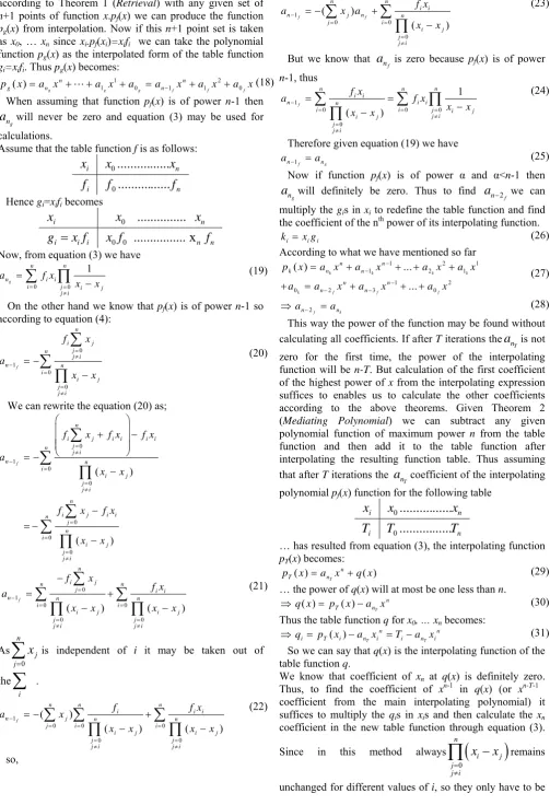
… has resulted from equation (3), the interpolating function pT(x) becomes:
( ) ( )
T
n
T n
p x a x q x (29)
… the power of q(x) will at most be one less than n.
( ) ( )
T
n
T n
q x p x a x
(30)
Thus the table function q for x0, … xn becomes:
( )
T T
n n
i T i n i i n i
q p x a x T a x
(31)
[image:3.595.49.553.54.791.2]So we can say that q(x) is the interpolating function of the table function q.
We know that coefficient of xn at q(x) is definitely zero.
Thus, to find the coefficient of xn-1 in q(x) (or xn-T-1 coefficient from the main interpolating polynomial) it suffices to multiply the qis in xis and then calculate the xn
coefficient in the new table function through equation (3).
Since in this method always
0 n
i j
j j i
x
x
remainscalculated once. Now given the above discussions we can offer the following simple algorithm for calculation of the coefficients of interpolating polynomial expressions:
0
0
1
0 ... {
( )
}
( 0 0) do{
0 ... {
. }
1 }
n
i i j
j j i
i
n i n
i i
n
n
i i i n i
k n
For i n do L x x end for
While k and f f a
L a For i n do
f x f a x end for
k k end while
B. The second method
Since the function pf(x) is of power n-1 and also given
Theorem 1 (Retrieval) we can find the pf(x) function from
re-interpolation for n given points. Also as the table function f coincides with pf(x) at n-1 point we can rule out
any given point and through interpolating of the remaining n points the same pf(x) will be produced again (This is in fact
another form of the RetrievalTheorem). Proof.
We assume that point xn is ruled out, now we want to
prove that 1 f
n
a
is produced from interpolation of the n remaining points. According to equation (24) we have:
1
0 0
1 1 1
0
0 0
1 1 1
0
0 0
1
1 1
( )
1 1
( )
f
n n
n i i
i j i j
j i
n n n
i i n n
i
j n j i n j i j
j i
n n n
i i n n
n n
i
j n j i n j i j
j i
a f x
x x
f x f x
x x x x x x f x x x f x
x x x x x x
with more expiation and rewriting;
1
0
1 1
1 1
0 0 0 0
1
1 1
( )
n
n n
j n j
n n
n n
i
i n
i j i j i i n j i j
j i j i
f x
x x
f
f x
x x x x x x
1 1
1 1
0 0 0 0 0
1
1 1
0 0 0 0 0
1 1 1
1 1 1
n n n
n n
i n n n i
i j i j j n j i j i j
j i j i
n n n
n n
i n n i
i j i j j n j i j i j
j i j n j i
f f x x f
x x x x x x
f x f f
x x x x x x
1 1
0 0 0 0
1 1
n n
n n
i n i
i j i j i j i j
j i j i
f x f
x x x x
therefore,
1 1 1
0 0
1
f f
n n
n i n n
i j i j
j i
a f x a x x
(32)On the other hand we know that f
n
a
is zero, so we have:1 1 1
0 0
1
f
n n
n i
i j i j
j i
a f
x x
(33)As there is no order among the points, whenever f
n
a
isproduced from equation (3) for n+1 points from the table function and is zero, we will be able to rule out any given point (e.g. xn) from the table function f and use the equation
(3) to calculate 1 f
n
a
, again. Now, fallowing T iterations thef
n T
a
coefficient is not zero for the first time, the power of the interpolating function would be n-T. Now we may subtractf
n T n T i
a
x
from the table function f for all points of x0, … xn-T-1 then use equation (3) to produce the coefficientof n T 1
x
for all points of x0, … xn-T-1. In this way, we mayoffer the following algorithm for calculation of coefficients in interpolating polynomial expressions:
0
0
0 ... {
( )
}
( 0 0) do{
0 ... ( 1) {
( )
} 1 }
n
i i j
j j i
i
n i n
i i
n
i i
i n
n
i i n i
For i n do L x x end do
While n and f f a
L a
For i n do L
L
x x f f a x end for
n n end while
IV. THE OTHER APPLICATION OF THEOREM 2 We may always add any given function of a polynomial g(x) with maximum power of n to fi expressions in such a
way that a number of fi+gis are would be zero. Then after
calculating the pf+g(x), the pf(x) will be produced through
subtracting g(x) from pf+g(x). On the other hand, when some
of fis are a fixed k number, if we choose g(x)=k (fixed
number) and subtract the table function fi we can reduce the
V. SOME EXAMPLES
(Example 1 for Mediating Polynomial theorem) We want to interpolate the following table function based on the Mediating Polynomial Theorem.
3 2 1 i
x
10 5 2 i
f
Assume that point (xi=1,fi=2) is a new added point and
polynomial for other two points (points 2 and 3) is driven out as g(x)=5(x-1). By subtracting g(x) from the new table function f we will have:
3 2 1 i
x
0 0 2 i i
g
f
Now we calculate the Lagrange Polynomial only for one point:
2
2 2
( 2)( 3)
( ) 2 5 6
(1 2)(1 3)
( ) ( ) ( ) 5 6 5 5 1
f g
f f g
x x
p x x x
p x p x g x x x x x
(Example 2) We need to calculate the interpolating function of the following table function based on the proposed algorithms.
0
x
1x
2x
3x
4x
i
x
0 1 2 -1 -2
1 2 15 0 -13 i
f
Solution based on the first method:
4
n
(Phase 1)
0 1 2 -1 -2
i
x
1 2 15 0
-13 i
f
4 -6 24 -6
24 i
L
1 4 2
6 15 24 0
6 13 24
i i
L
f
4 4
0
0
f
i
i i
f a
L
(Phase 2)
5
. (0)
i i i
f x f x
0 1 2 -1 -2
i
x
0 2 30 0
26 i
f
4 -6 24 -6 24
i
L
0 4 2
6 30 24 0
6 26 24
i i
L
f
4 3
0
2
f
i
i i
f a
L
(Phase 3)
5
. (2)
i i i
f x f x
0 1 2 -1 -2
i
x
0 0 -4 2
12 i
f
4 -6 24 -6 24
i
L
0 4 0
6 4 24 2
6 12
24
i i
L
f
4 2
0
0
f
i
i i
f a
L
(Phase 4)
5
. (0)
i i i
f x f x
0 1 2 -1 -2
i
x
0 0 -8 -2 -24
i
f
4 -6 24 -6 24
i
L
0 4 0
6 8 24 2 6 24 24
i i
L
f
4 1
0
1
f
i
i i
f a
L
(Phase 5)
5
. ( 1)
i i i
f x f x
0 1 2 -1 -2
i
x
0 1 16 1
16 i
f
4 -6 24 -6
24 i
L
0 4 1
6 16 24 1
6 16 24
i i
L
f
4 0
0
1
f
i
i i
f a
L
Thus the interpolating function becomes:
4 3 2 3
4 3 2 1 0
( ) 2 1
f f f f f
f
p x a x a x a x a xa x x
Solution based on the second method:
4
n
(Phase 1)
0 1 2
-1 -2
i
x
1 2 15 0
-13 i
f
4 -6 24 -6
24 i
L
1 4 2
6 15 24 0
6 13 24
i i
4 4
0
4 4
0
( )
(0)
i
i i
i i
i
i i i
f a
L L L
x x f f x
Delete x4n=3
(Phase 2)
0 1
2 -1
-2 i
x
1 2
15 0
i
f
2 -2
6 -6
i
L
1 2 2
2 15
6 0
6
i i
L
f
3 3
0
3 3
2
( )
(2)
i
i i
i i
i
i i i
f a
L L L
x x f f x
Delete x3n=2
(Phase 3)
0 1
2 -1
-2 i
x
1 0
-1 i
f
2 -1
2 i
L
1 2 0
1 1
2
i i
L
f
2 2
0
2 2
0
( )
(0)
i
i i
i i
i
i i i
f a
L L L
x x f f x
Delete x2n=1
(Phase 4)
0 1
2 -1
-2 i
x
1 0
i
f
-1 1
i
L
1 1 0
1
i i
L
f
1 1
0
1 1
1
( )
( 1)
i
i i
i i
i
i i i
f a
L L L
x x f f x
Delete x1n=0
(Phase 5)
0 1
2 -1
-2 i
x
1 i
f
1 i
L
1 1
i i
L
f
0 1
0
1
i
i i
f a
L
Thus the interpolating function becomes:
4 3 2 3
4 3 2 1 0
( ) 2 1
f f f f f
f
p x a x a x a x a xa x x
VI. CONCLUSION
We’ve presented here two new algorithms based on Lagrange interpolation formula to calculate coefficients of polynomial. Two theorems are presented here. The main objective of this paper is, however polynomial coefficients calculation, the second theorem (Mediating Polynomial) is applicable for updating systems. When a new point is added to the table, it is just needed to calculate the polynomial for the new point, by using the Mediating Polynomial theorem and updating the coefficients.
REFERENCES
[1] Trefethen, Lloyd N. Approximation theory and approximation practice (Book style). Siam, 2013, pp. 3.
[2] Van Beeumen, Roel, Wim Michiels, and Karl Meerbergen, “Linearization of Lagrange and Hermite interpolating matrix polynomials.” IMA Journal of Numerical Analysis, 2014, dru019. [3] Berrut, Jean-Paul, and Lloyd N. Trefethen, “Barycentric Lagrange
interpolation,” Siam Review. Vol. 46, no. 3, 2004, pp. 501-517. [4] Werner, Wilhelm, “Polynomial interpolation: Lagrange versus
Newton,” Mathematics of computation, vol. 43, no. 167, 1984, pp. 205-217.
[5] Feng, Yong, Xiaolin Qin, Jingzhong Zhang, and Xun Yuan, “Obtaining exact interpolation multivariate polynomial by approximation.” Journal of Systems Science and Complexity. Vol. 24, no. 4, 2011, pp. 803-815.
[6] Solares, Cristina, Eduardo W. Vieira, and Roberto Mínguez, “Functional networks and the lagrange polynomial interpolation.”
In Intelligent Data Engineering and Automated Learning–IDEAL,
Springer Berlin Heidelberg, 2006, pp. 394-401.