Abstract— Policing approaches to patrolling and response to incidents can be more effective if predictive policing is used to make decisions. Predictive policing uses information such as historical crime data to predict crime patterns and response demand. This information can then be used to direct resources more efficiently. This research develops a method of response officer patrol route planning based on predictive policing. Historical crime and call data is used to anticipate the levels of response demand and to identify high crime areas and to determine the best locations to position resources. This study shows how kernel density estimation is used for crime mapping and a maximum coverage location problem is formulated to maximize demand coverage. This is then solved using exhaustive search and tabu search. Tabu search gave sub-optimal results but gave significant reductions in computational time compared to exhaustive search.
Index Terms—Police response, hotspots, maximum coverage location problem, tabu search, exhaustive search
I. INTRODUCTION
HE police response service has a duty to respond to incidents which require a timely attendance at the scene. This service is vital to the safety of the public but is constantly challenged by the limited resources available due to funding cuts to the entire police force. A decrease in resources cannot lead to a decrease in the effectiveness of this service as this could compromise the public’s safety. Hence methods to improve the effectiveness of the available resources are required.
Two ways in which the response service can be improved are to reduce crime levels and to anticipate possible response demand, where response demand is the predicted levels of calls requiring an officer presence at the scene. It has been proven that targeting problem areas, hotspots, can reduce overall crime levels [1] - [3]. In this research kernel density estimation [4] is used to identify hotspots and these are used to position response officers to target these problem areas. To anticipate possible response demand, historical data can be analyzed. These two factors can be used to determine the optimal positioning of police response officers. The importance of effective deployment of
Manuscript received December 29, 2015; revised January 20, 2016. This work was supported by the Economic and Social Research Council ES/K002392/1.
J. M. Leigh is with the Aeronautical and Automotive Engineering Department, Loughborough University, Loughborough, LE11 3TU, UK (phone: 01509 227264; e-mail: [email protected]).
S. J. Dunnett is with the Aeronautical and Automotive Engineering Department, Loughborough University, Loughborough, LE11 3TU, UK (phone: 01509 227258; e-mail: [email protected]).
L. M. Jackson is with the Aeronautical and Automotive Engineering Department Loughborough University, Loughborough, LE11 3TU, UK (phone: 01509 227276; e-mail: [email protected]).
resources in a time of depleting resources is outlined in [5]. The positioning program developed uses the hotspots identified, within the maximum coverage location problem (MCLP), to identify the hotspots which officers should be sent to whilst patrolling in order to provide the best demand coverage. The MCLP technique used here considers covering city and rural demand with different time constraints.
The layout of the paper is as follows: Section ІІ discusses the background to the work and reviews some of the studies which have helped progress innovation in this field. Section ІІІ describes the problem to be solved. Section ІV details the methods of crime mapping. Section V describes the use of MCLPs to determine the best positioning of officers to give optimal demand coverage. Section VІ describes the methods used for solving the MCLP. Section VІІ gives preliminary results and section VІІІ concludes the outcomes of this research and identifies future directions.
II. BACKGROUND
Police officers in response have the main task of attending to incidents. Whilst officers are not attending to incidents their role is to provide a community presence by patrolling high crime areas. With many police forces these areas are decided by the officer using information given to them during briefings at the beginning of their shift. The information usually includes way markers which are areas of concern selected on a map by crime analysts. This research advances this process through combining targeting hotspots with demand data to determine in real time the best positioning for police officers.
Previous studies on patrol routing include [6] and [7]. Reference [6] develops a tool, GAPatrol, to help police managers plan patrol routes. In this study multiagent-based simulation assists in the design of police patrol routes. The simulation finds crime hotspots and plans routes with better attendance to these hotspot areas. Hence the routes are planned with the single aim of reducing crime levels and do not consider demand coverage for incident response.
In [7] patrol routes are planned based on giving each road a crime rating and visiting those with the highest costs whilst also keeping cost of travel low. This study does not consider demand coverage for incident response and also only considers one police unit at a time which is not practical. In reality there are many units and where each of these units is patrolling effects the other units.
There have been many studies on identifying hotspots, these have been used to develop the method of hotspot mapping which is part of the positioning process. There has also been research on using demand to position emergency
Predictive Policing Using Hotspot Analysis
Johanna M. Leigh, Sarah J. Dunnett, and Lisa M. Jackson
services vehicles such as police and ambulances. Both of these research areas relate to the positioning system developed here and hence have been considered in detail.
A. Hotspots
Hotspot mapping is a method of using past incident data to predict future crime patterns. These patterns emerge due to the location of crimes not being random. The location of crimes is dependent on the geographical layout of the area [8]. Hotspot mapping is a popular method used within the police force as well as other law enforcement services. One use of this technique was by West Midlands Police during Operation SAVVY [2]. This study identified 150m2 hotspots and targeted those using police community support officers for fifteen minute periods, three times during peak crime periods. The outcome of this study was a reduction in crime in medium and high level crime areas. This proves that targeting crime hotspots is an effective way of reducing overall crime. Reference [3] compares police randomized control trials which use hot spots to focus police action towards. The outcome of this study showed that hot spot targeting does reduce overall crime levels and not just a displacement of crimes.
Methods of identifying hotspots include point mapping, spatial ellipses, thematic mapping for geographical areas or a grid, and kernel density estimation. The point map plots the crimes on the map as points and then the distribution of these points is observed. This method is simple and dated, it was used in the early days of predictive policing, since then methods have been advanced. Spatial ellipses find the areas with the highest crime densities, and then plots a standard deviation ellipse over these areas, each ellipse is considered to be a hotspot. This method has been used frequently in studies, one example is analyzing the effect of school holidays on crime distribution in The Bronx, New York [9]. The benefit of this method is that it doesn’t use boundaries. The issue is that crime patterns don’t always form ellipses. The thematic mapping approach either divides the map into geographical areas, such as census areas or police beat boundaries, or places a grid over the map. The areas or grid cells are then shaded in a color to represent the number of crimes which occur in that area. The hotspots are determined by deciding a threshold value above which the areas are considered to be hotspots. In [10] a limit of 3% of the total area to be considered is set as hot, hence the highest 3% of crime levels were set as hotspots. The use of geographical boundaries as dividers results in areas of unequal size. Comparing regions of unequal size can lead to misconceptions about crime rates in areas and hence is not the best method to determine hotspots. This method is still used for applications such as analysis and visual representation of crime patterns and auditing across partnership administrative zones, [11]. Grid thematic mapping solves the problem of unequal region sizes by placing a uniform grid over the map. An acceptable grid cell size is found through testing, [10] used a grid cell size of 250m and [8] used a grid cell size of 200m. An example of when thematic mapping has been used is for the analysis of distribution of emergency calls and violent offences, [12]. Kernel density estimation is widely used within police crime
analysis to identify hotspots. It has good spatial analysis and visualization properties which have proved useful to the police [10] and [13]. It represents crime distribution as a smooth continuous surface [14]. A grid is still used in the calculation process and grid cell size and bandwidth are required, these are determined depending on the application. A study into the ability of each of the methods mentioned above to predict future crime locations was carried out by [10]. Kernel density estimation proved to be the best method of predicting future crime patterns. The study also showed that street crime locations are predicted more accurately from historical data than residential burglary, or theft from or of a vehicle.
B. Maximum Coverage Location Problem
For the police response positioning problem, a finite number of police officers are required to patrol a finite number of hotspots in a way that maximizes the demand coverage, hence this problem can be solved as a MCLP. Other dispatch problems which have previously been solved as MCLPs include ambulance and fire-engine dispatch.
Ambulance MCLPs include [15]-[17]. [15] uses a simple MCLP equation to determine the places to locate ambulances. The locations considered are ambulance bases such as fire stations and service stations. This is solved as a stationary problem, it does not consider repositioning when other ambulances are moved. It was a basis for solving many other MCLPs for ambulances. Reference [16] develops the double standard model which advances on [15] by considering two time restrictions, one which meets response targets and another which does not for when it is not possible to meet the response targets. This means the system allows for a certain percentage of responses to be covered outside of response limits. It also considers that some areas require higher coverage than other areas. This is important to the police response positioning problem, as in high demand areas one officer presence cannot cover all demand. Response demand levels vary depending on geographical location hence emergency demand levels also vary. Reference [17] considers that ambulances will be moved during a shift hence repositions the remaining resources in the event of an incident. When repositioning the ambulances this study takes into account server availability and two different types of server. The server availability is an area which must also be considered when dealing with police officers.
The hotspot identification and MCLP discussed here are used to solve the police response officer positioning problem.
III. PROBLEM FORMULATION
must take the crime data, filter this data to only the necessary and accurate data, and then use this to find hotspots on a regular basis. These hotspots can then be used, along with the resource list and predicted response demand data, in the MCLP to find the most effective hotspots to send resources too. The resources which can be positioned are those which are available. Officers attending to incidents will add to the demand coverage but will not be included in the repositioning. Once the solution is found officers will be given a hotspot location along with the major crimes which occur within this hotspot to allow them to target the problem. Activities based on targeting these crimes can be given to the officers by the police force. This can include door knocking in high burglary rate areas.
[image:3.595.59.270.270.436.2]The area used as a case study within this study is Leicestershire Police. Data from OpenStreetMap [18] was used to form a road map of the area shown in Fig. 1.
Fig. 1. Road map of Leicestershire
IV. CRIME MAPPING
Crime levels are dependent on geography as geographical markers effect criminal’s decisions. This results in spatial patterns forming. Proof of crime patterns being formed due to criminal decisions is shown in [19].
A. Data Filtering
Not all the crime data is accurate and not all data is relevant. Initial filtering will filter out inaccuracies. The next stage is to filter out irrelevant information. Not all crimes are deterred by the presence of an officer on the street hence targeting these crimes with patrols would not be effective.
0 5 10 15 20 25
0 1 2 3 4 5 6
Crimes Depending on Day of the Week and Hour
Hour
C
ri
m
e Lev
el
Friday
Sunday Wednesday
Saturday Thursday
Monday
Tuesday Sunday
Monday Tuesday Wednesday Thursday Friday Saturday
Fig. 2. Variation in ASB over time.
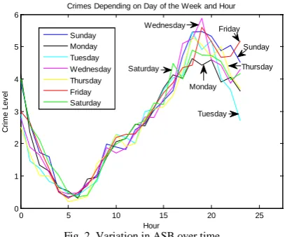
Those crimes which are deterred and will be included in the hotspot identification are anti-social behavior, theft, vehicle theft or theft from a vehicle, burglary including in dwelling and criminal damage. Incidents which occur in certain places such as clubs/bars, shopping centers and hospitals are not affected by patrols and are not included in the analysis.
[image:3.595.311.533.441.615.2]As crime levels are not constant the data also has to be broken down by time, day and season for analysis. This has been achieved using kernel density estimation in this work. Fig. 2 shows how anti-social behavior (ASB) crime levels vary over time and day.
B. Quadratic Kernel Density Estimation
There are many different methods of identifying crime hotspots. Kernel density estimation (KDE) has proven to have the best prediction qualities by [10]. This method finds crime patterns by looking at crimes and the surrounding area. This reduces the effect of boundaries on the analysis as the inclusion of boundaries, such as town boundaries, may not allow hotspots to be identified accurately as hotspots lying across the boundary would not be considered. Quadratic kernel density estimation (QKDE) uses a grid whilst also taking into account the crimes in the area around the grid cell.
QKDE is demonstrated in Fig. 3. Firstly a grid is overlaid onto a crime map. Then each grid cell is considered and KDE performed. KDE looks at the crimes within a certain bandwidth from the center of the grid cell and uses an equation, such as that shown in equation (1), to determine the intensity of crime within that grid cell. Equation (1) is taken from [20], and is specific for use in crime analysis.
Fig. 3. QKDE diagram.
( )
32 1 22 2ˆ
−
=
∑
≤ πτ τ λ
τ
τ i
d
d s
i
(1)
Where λˆτ
( )
s is the intensity of crimes within thebandwidth radius (τ) as a function of the distance from the grid center (s). di is the distance between s and the point being investigated.
[image:3.595.71.275.611.780.2]and grid cell size 0.001ο x 0.001ο, measured in the longitude and latitude coordinate system.
V. MAXIMUM COVERAGE LOCATION PROBLEM
Now the possible locations to position officers have been found, by crime mapping, the most appropriate ones to visit need to be selected. This is done by calculating which layout creates the optimal demand coverage. Demand is the level of calls which require attendance in each area. Coverage is whether an officer can reach the demand within the response times. These response times are different for different police forces. Typically for emergency response there are two response time standards tc and tR, one for city and town centers and another for rural areas. This is due to quicker response times expected in highly populated areas such as city and town centers than in low populated areas such as rural areas. In Leicestershire the city response time target is below fifteen minutes and in rural areas is below twenty minutes.
The MCLP uses hotspots as possible officer locations. These are represented by the set of points
{
w w wm}
W = 1, 2,2, where m is the total number of
hotspots. The demand points are represented by the set
{
v v vn}
V = 1, 2,2, where n is the total number of demand points. The demand points are found by overlaying a grid on the map and then determining how many emergency calls originate from each grid cell.
The MCLP used here is a variation of the double standard model used for ambulance dispatched [16]. The objective function is shown in (2). The equation represents demand at a node i by
i
d and uses xik to indicate whether i is covered by an officer. xik is a binary number which equals 1 if vi is covered a minimum of k times within radius r1 by officers and 0 if it is not covered.
( )
∑
∈V i
k i i x
d
Maximise (2)
This objective function does not consider the city and rural area time standards. When determining if demand is covered these rules must be included:
• when considering a town/city a unit must be located such that it could reach node i within tc, to be considered covered
• when considering a rural area a unit must be located such that it could reach node i within tR, to be considered covered
To incorporate these into the problem the time standards are considered as distances where r1 is the distance which can be travelled within tc and r2 is the distance which can be travelled within tR. The objective function is shown in (3), it is split into city and rural response by the use of C and R which are binary values where 1 represents the area being within that classification and 0 the area is outside that classification. 1xik is a binary value which equals 1 if vi is covered a minimum of k times within the radius r1. 2xik is a binary value which equals 1 if vi is covered a minimum of k times within the radius r2.
(
)
∑
∈
+
V i
k i i k i
i x C d x R
d
Maximise 1 2 (3)
The objective function is subject to the constraints
(
i V)
y
k i
W j
j ≥ ∈
∑
∈
1 (4)
(
v V)
x xik+1≤1,2 ik i∈
2 ,
1 (5)
∑
∈ =
W j
j p
y (6)
{ } (
v V)
x
x k i
i k
i , 2 ∈ 0,1 ∈
1 (7)
{ }
0,1 ,R∈C (8)
1 =
+R
C (9)
2 1 r
r < (10)
yj shows the number of resources located at j. The total number of units available is taken to be p and this is determined by the number of officers on shift with an available status at that time, whether they are single or double crewed. The solution will aim to cover all demand within at least
2
r which is taken into account by constraint (4) which states all demand should be covered. Constraint (5) states that node i can only be covered k+1 times if it is covered at least k times. Constraint (6) ensures that the sum of all the officers at each point W is equal to p. Constraint (7) and (8) ensures 1xi
k , 2xi
k
, C and R are binary numbers. Constraint (9) states that either C or R must equal 1, but never both at the same time. The final constraint (10) ensures that the distance travelled within the city response time is smaller than the distance which can be travelled with the rural response time.
VI. SOLVING
When solving the objective function there are rules on where each officer can be placed due to their status and attached station. These are:
1. An officer can only move if its status is available (e.g. if they are not attending an incident, in custody or on a break).
2. An officer only counts as covering an area if they are free to attend an emergency incident, this includes officers who are available, on a break or attending an incident more minor than an emergency incident.
Rule 1 is just the condition that a police officer must be available before moving them. In rule 2 an officer is counted as covering an area if attending a grade 2 incident because if necessary they can leave such an incident to respond to an emergency incident but they cannot be moved unnecessarily. Hence they are not moved when solving for maximum coverage. Rule 3 ensures that officers do not move too far from their base police station. Each officer has an attachment to a particular police station and even though the aim is for police forces to operate as boundaryless within their region it is not efficient to move an officer too far away from their associated station due to their journey back at the end of a shift.
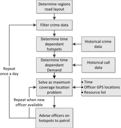
The objective function is solved on more than one occasion. The flow chart in Fig. 4 shows the process the system runs though. It demonstrates that the solving is repeated when new officer’s become available. Also once a hotspot has been visited for the allocated time period, typically 10-15 minutes, the officer becomes available again.
Determine regions road layout Filter crime data
Determine time dependant
hotspots
Solve as maximum coverage location
problem
Advise officers on hotspots to patrol
• Time
• Officer GPS locations
• Resource list Historical crime
data
Repeat when new officer available Repeat
once a day
Determine time dependant
Demand
[image:5.595.62.275.287.512.2]Historical call data
Fig. 4. Flow chart of positioning system process
Initially solutions are found using exhaustive search where each solution is investigated and the optimal solution is then found. This is process has a high computational time which may not be suitable in the real world situation. Tabu search is also be used to solve the objective function. The computational time of this method is lower as not every solution is explored. This means the optimal solution is not guaranteed. The results are then compared to determine whether Tabu search is sufficiently accurate to be used in real time.
The Tabu search cuts down the search area by basing which possible solution to investigate next on the results of previous solutions and then using stopping criteria to halt the search before every solution is explored [21]. The search process is called neighborhood search. Initially a feasible solution is selected and solved to find the demand coverage value, f*. Then the objective function is then solved for the neighbors, N(S), of this original solution. A neighbor is where there is one move difference between it and the previous solution. The method then chooses the best, S*, out
of the neighboring solutions. This solution is then the current solution, S, which is used to base the next solutions on. The best is classified as which solution maximizes the objective function, argmax[f(S’)], i.e. gives the highest demand coverage. The method allows solutions worse than the previous solution to be chosen to stop the search getting stuck at a local optima. The search will continue until one of the stopping criterions is met.
The stopping criteria are:
• there has been no improvement in the solution since a set number of iterations
• the maximum set number of iterations has been met • the optimal solution is found.
To stop repeat visiting of solutions a tabu list is formed, which visited solutions are placed on for a set number of iterations.
Once the officers have visited a hotspot the effect lasts after the officer leaves. This means repeat visiting within close time periods is not effective. To stop repeat visiting of hotspots a tabu list with a longer memory is formed to stop hotspots being included in solutions. This tabu list memory will last across multiple searches until the hotspot requires revisiting.
VII. RESULTS
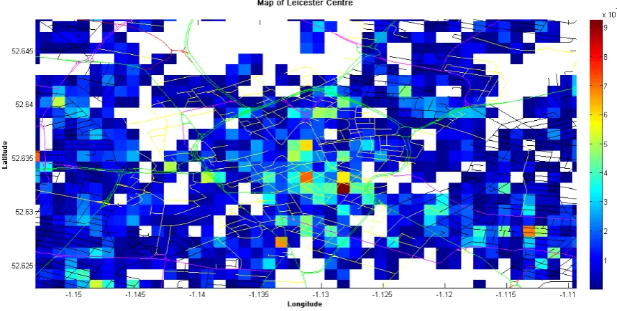
The result of this work is a process which automatically allocates officers to efficient patrolling locations. The kernel density estimation analysis identified hotspots. An example of a graph produced is shown in Fig. 5. This shows criminal damage hotspots. The shaded areas show where crimes have taken place. The color bar on the left of the graph shows the highest crime intensity at the top and the lowest crime intensity at the bottom. No color means there were no relevant cases of criminal damage. Each type of crime contributes to the overall hotspots.
Out of the area analyzed 3% of the area is classed as hotspots. Hence the grid cells with the top 3% of intensity are considered as hotspots in the MCLP.
The hotspots are then used to solve the MCLP to find where response officers should be located. Table I gives the average time taken to perform exhaustive search and the time taken to perform tabu search along with the demand coverage achieved by each method.
The table shows that the time to perform exhaustive search is significantly higher than for tabu search. Hence the computational time can be cut drastically using tabu search within the positioning process. The table also shows that exhaustive search produces higher demand coverage on average. This is due to exhaustive search always finding the optimal positioning and tabu search not guaranteeing the optimal positioning. Tabu search can choose positioning which is only close to optimal. In this case the difference in
TABLEI
RESULTS OF EXHAUSTIVE AND TABU SEARCH
Search Method Time (s) Demand Coverage
Exhaustive 323 4.48
[image:5.595.317.551.741.781.2]Fig. 5. Hotspots for anti-social behaviour
demand coverage between exhaustive search and tabu search was 1.3% and this is considered to be sufficiently accurate to base patrolling on and is necessary when considering the time constraints of the process.
VIII. CONCLUSION
Using predictive policing can improve the quality of service by preventing crime and placing resources in a good position to react to incidents. Directing patrol routes in real time can lead to more efficient crime targeting as well as real time positioning for demand.
The tabu search saved computational time with insignificant effects to the demand coverage. Using Exhaustive search found the optimal solution but is not suitable for use within the real time problem solving due to the speed at which an a solution is required.
Future work on this project should involve allocating particular activities to hotspots which target the main crimes in that area. An area for future work is accounting for the harm caused by each crime to develop hotspots weighted on the severity of the crime. This would align with current pushes to rate police standards based on harm caused by incidents.
ACKNOWLEDGMENT
The cooperation of the Leicestershire Police is gratefully acknowledged as without this support this project would not be possible.
REFERENCES
[1] J. Smallwood, 2015. What Works Crime Reduction: Operation SAVVY. College of Policing. Available:
http://whatworks.college.police.uk/Research-Map/Pages/ResearchProject.aspx?projectid=306.
[2] D. Weisburd and T. McEwen, “Introduction: Crime mapping and crime prevention,” in New York: Criminal Justice Press, pp 1-23, 1997.
[3] A. Braga, “Hot spots policing and crime prevention: a systematic review of randomized controlled trails,” in Journal of Experimental Criminology, Springer, 2005, issue 1, pp. 317-342.
[4] J. Eck, S. Chainey, J. Cameron, M. Leitner, and R, Wilson, “Mapping crime: understanding hot spots,” in National Institute of Justice, 2005, pp. 26-33.
[5] C. McCue, Data Mining and Predictive Analysis: Intelligence Gathering and Crime Analysis, Butterworth-Heinemann as an imprint of Elsevier, 2007, pp. 239-241
[6] D. Reis, A. Melo, A. Coelho, and V. Furtado, “Towards optimal police patrol routes with genetic algorithms,” in Mehrotra, Springer, 2006, vol. 3975, pp. 485-491.
[7] S.S. Chawathe, “Organizing hot-spot police patrol routes,” in
Intelligence and Security Informatics, IEEE, 2007, pp.79-86.
[8] S. Chainey and J. Ratcliffe, GIS and Crime Mapping, Wiley, London, 2005, chapter 4.
[9] R. Langworthy and E. Jefferis. “The utility of standard deviation ellipses for evaluating hotspots,” in Analyzing Crime Patterns: Frontiers of Practice, 2000, pp. 87-104.
[10] S. Chainey, L. Tompson and S. Uhlig, “The utility of hotspot mapping for predicting spatial patterns of crime,” in Security Journal, Palgrave Macmillan. 2008, vol. 21, pp. 4-28.
[11] N. Levine, “Crime mapping and the Crimestat program” in Geographical analysis, 2006, vol. 38, issue 1, pp. 41-56.
[12] S. Chainey, “Combating crime through partnership; Examples of crime and disorder mapping solutions in London, UK,” in Mapping and Analysing Crime Data: Lessons from Research and Practice, Taylor and Francis, New York and London, 2001.
[13] J. LeBeau, “Mapping out hazardous space for police work,” in Mapping and Analysing Crime Data. Taylor and Francis, London and New York, 2001, pp 138-155.
[14] T. Hart and P. Zandbergen, “Kernel density estimation and hotspot mapping,” in Policing: An International Journal of Police Strategies & Management, 2014, vol. 37, issue 2, pp. 305-323
[15] M. Daskin, “A hierarchical objective set covering model for emergency medical service vehicle deployment,” in Transport Science Institute for Operational Research and the Management Science, vol. 15, no. 2, pp. 137-152.
[16] M. Gendreau, G. Laporte, F. Semet, “Solving an ambulance location model by tabu search” in Location Science, vol. 5, no. 2, pp. 75-88. [17] M. Mandell “Covering models for two-tiered emergency services
systems” in Locations Science vol. 6, pp. 355-368, 1998.
[18] OpenStreetMaps & Contributors, Maps, 2015 Available: http://www.openstreetmap.org/. Last accessed 01/09/2014
[19] D. Reis, A. Melo, A. Coelho and V. Furtado, “Towards optimal police patrol routes with genetic algorithms,” in Mehorta, vol. 3975, pp. 485-491.
[20] A. Gatrell, T. Bailey, P. Diggle and B. Rowlingson, “Spatial point pattern analysis and its applications in geographical epidemiology,” in Transactions of the Institute of British Geographers, vol. 21, no. 1, pp. 256-274.