Abstract— This research aims at of the polyethylene extrusion process in plastic industry using the framework of Process Analytical Technology (PAT) utilizing fuzzy-neural approach. Two pipe's quality responses, weight, and thickness where chosen as both are main features of manufacturer interest. Initially, the individual moving range (I-MR) control charts are established for each response which illustrates that the process is incapable. Nine process factors are studied utilizing the L27 array. The fuzzy-neural approach is, therefore, proposed and then implemented to optimize process settings. Confirmation experiments are finally conducted at the combination of optimal factor settings. It is found that the estimated mean values for weight and thickness are close to their corresponding targets. Moreover, the estimated standard deviations for the pipe's weight and thickness are reduced significantly using the optimal factor settings. As a result, the estimated process capability indices are significantly enhanced for both responses.
Index Terms—PAT Framework, Extrusion Process, Process Capability, Multiple Responses.
I. INTRODUCTION
Due to inexpensive raw materials, ease of processing, greater flexibility in the design of components, and attractive properties, the demand for plastic products has dramatically increased. In such products in order to meet customer expectations, manufacturers should continually optimize plastic manufacturing processes in a cost-effective manner [1-2]. Among the heavily-used plastic products is the Unplasticized Poly Vinyl Chloride (uPVC) pipe used in pressure and non-pressure applications; such as, transfer water, protection electrical, communications wires and other applications. The main manufacturing processes involved in producing uPVC pipes are the injection and extrusion processes. In order to cut huge quality costs, optimizing the performance of plastic process becomes a real challenge to product/process engineers.
A. Process Analytical Technology
Process Analytical Technology (PAT) is a system for designing, analyzing, and controlling plastic manufacturing through timely measurements of critical quality and performance attributes of raw and in-process materials and processes, to ensure final product quality [3-4]. The PAT’s goal is to enhance the understanding and controlling of the manufacturing process to improve quality and efficiency.
Manuscript received Feb. 20, 2017; revised April,10, 2017.
A. Al-Refaie is with the University of Jordan (corresponding author e-mail: abbas.alrefai@ ju.edu.jo).
N. Bata received master degree in industrial Engineering from the University of Jordan.
B. Fuzzy logic
[image:1.595.322.530.303.422.2]
Typically, the fuzzy logic principle is widely-applied to deal with vague and unsure information for optimizing performance using multiple quality characteristics [5]. The Mamdani systems in fuzzy logic involve mathematical expressions that have a linear function [6]. Generally, a fuzzy system shown in Fig. 1 includes the fuzzifier, fuzzy rules, and the defuzzifier that transforms the fuzzy input values into a comprehensive output measure [7].
Fig. 1. A schematic of fuzzy logic system.
C. Artificial Neural Networks
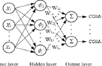
The Artificial Neural Networks (ANNs) are soft computing techniques used to emulate some functions of the human behavior, by having a finite number of layers with different neurons being as the computing elements [8]. The most popular type of ANNs consists of input, hidden, and output layers. The input and output layers represent the nodes, and the hidden layer represents the relationship between the input and output layers. In ANNs, the Radial Basis Function Neural Network (RBFNN) shown in Fig. 2 can approximate the desired outputs predicted without a need to have a mathematical formula of the relationship among the outputs and the inputs [9].
Fig. 2. Architecture of the RBFNN.
Abbas Al-Refaie and Nour Bata
[image:1.595.350.515.632.739.2]Previous research attempted to improve uPVC pipes' quality and enhance extrusion process's productivity. For example, Mu et al. [10] developed an optimization approach for processing design in the extrusion process of plastic profile with metal insert. Mamalis et al. [11] optimized processing parameters of Tube -extrusion of polymeric materials. This research utilizes the fuzzy logic and RBFNN techniques in the PAT framework to optimize the parameters of plastic extrusion process. Research results may contribute to reduce huge quality and production costs.
II. MATERİALS AND METHODS
The pipes' manufacturing line starts by mixing the raw material, which consists mainly of uPVC particles. Within the barrel, raw material is subjected to extremely high temperatures until it starts to melt. Depending on the type of thermoplastic, barrel temperatures can range between 400 and 530 degrees Fahrenheit. Once the molten plastic reaches the end of the barrel, it is forced through a screen pack and fed into the feed pipe that leads to the die, which is designed and built based on the dimensions desired in the pipe and the shrink rate of the type of plastic being used. After leaving the extrusion die, the pipe passes through precision sizing sleeves with an external vacuum. The puller or haul off is used to pull off the pipe through sizing and cooling operations. To expedite the cooling process, the newly formed plastic receives a sealed water bath. Once it has passed a certain length, it will trip a sensor (electric eye) triggering a cutting operation on the pipe. The cut is made by a cutter that moves forward at the rate of pipe extrusion to offset the motion of the pipe moving forward so that the end of the pipe will remain perpendicular to the pipe wall after it is cut. The PAT framework is then implemented as follows.
i. Identifying critical process attributes
The pipe quality can be described by several physical parameters; such as, accurate pipes weight and thickness. Pipe's average thickness and average weight are considered the most vital quality characteristics. Typically, the pipe is composed of PVC and additives, such as UV inhibitors, anti-oxidants, or colorants. Accurate pipe's weight for a homogeneous powder mixture ensures that each produced pipe contains sufficient amount of resin stated in the standards. The specification of the pipe’s weight is 1666 ± 14 grams/meter. Thus, the average weight is considered as nominal-the-best (NTB) type. The thickness is also a significant measure to the uniformity of the pipe and the resulted defects; an accurate thickness is an indicator to a good surface finish. Therefore, pipe's thickness will be used as an indicator to measure if it can hold the pressure on its' inner wall and does not cause pipe's fracture. The specifications of the pipe's thickness are 3200 ± 200 Micrometer. The pipe thickness is measured using a Vernier caliper, while the pipe weight is measured using a weighing device.
ii. Real-time monitoring
A control chart is one of the primary monitoring techniques of statistical Process control. A normality test for the current
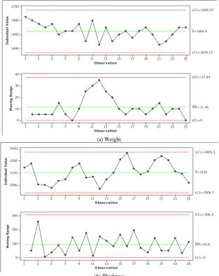
data is conducted before proceeding in establishing the control charts. The p values of 0.379 and 0.857 are found for the pipe's average weight and thickness, respectively, which confirms that the normal distribution is a satisfactory model for each response. The data is collected for the pipe's thickness and weight. I-MR control charts for the averages of pipe's weight and thickness are constructed and depicted in Fig. 3. In this figure, the calculated LCL, CL, and UCL
values for I chart are 1634.13, 1664.6, and 1695.07 g/m, respectively, while their respective values for the MR chart are estimated 0.0, 11.46, and 37.44 g/m. For the average thickness, the LCL, CL, and UCL of the I chart are respectively calculated as 2906.7, 3156.0, and 3405.3 µm, while their values for the MR chart are estimated 0.0, 93.8, and 306.4 µm, respectively. Observing the I-MR charts, neither point falls beyond the control limits nor is a significant pattern observed within the control limits for both the pipe's average weight and thickness. Consequently, the I-MR charts are concluded in statistical control.
A vital part of an overall quality-improvement program is the process capability analysis by which the capability of a manufacturing process can be measured and assessed. The
p
C is estimated as shown in Eq. (1). ˆ
ˆ 6 p
USL LSL
C
(1)
Furthermore, the actual process capability index, Cpk, attempts to take the target, T, into account. The actual capability index,
pk
C , can be expressed mathematically by: ˆ ˆ
ˆ min ,
ˆ ˆ
3 3
pk
USL LSL
C
(2) A criterion for selecting an optimal design is known asMCˆpkand is used as a capability measure for a process having multiple performance measures. ˆ
pk
MC is a proposed system capability index for the process which is the geometric mean of performance measure ˆ
pk
C values.
1
1
ˆ ˆ
m
m pk pki
i
MC C
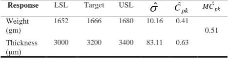
(3)where m is the number of quality characteristics. A summary of all the statistical data gathered in the
[image:2.595.310.544.630.691.2]measuring phase for both quality characteristics is listed in Table 1.
Table 1. Statistical summary for both quality responses.
Response LSL Target USL
ˆ
ˆpk
C MCˆpk
Weight (gm)
1652 1666 1680 10.16 0.41
0.51
Thickness (μm)
3000 3200 3400 83.11 0.63
In Table 1, it is found that the process is found incapable for both responses. Therefore, process optimization is required.
iii. Optimization and Prediction
are the nominal-the-best (NTB) type responses. Based on technical knowledge, nine three-level process factors are studied. The appropriate array is the L27 orthogonal array
[image:3.595.68.269.115.229.2]shown in Table 2.
Table 2. The controllable factors and their levels.
Process factor Level
1 2 3
x1: T1 (˚C) 190 195 200
x2: T2 (˚C) 180 185 190
x3: T3 (˚C) 165 170 175
x4: T4 (˚C) 165 170 175
x5: T5 (˚C) 160 165 170
x6: T6 (˚C) 170 175 180
x7: T7 (˚C) 165 170 175
x8: T8 (˚C) 225 230 235
x9: Screw speed (rpm) 700 800 900
In the Taguchi method, the orthogonal array (OA) consists of columns that represent the controllable factors to be studied. While, the rows represent the combination of factor levels at which experiments are held. Let ij denotes the signal-to noise ratio for the jth response at experiment i
calculated for the nominal-the-best (NTB) type response as:
2 2
10 log[ / ] ; 1,..., 27
i yi si i
(4) where
_
i
y and
s
i are the estimated average and standard deviation in experiment i of each response, respectively. In this research, nine three-level factors are considered, and thus the L27 array shown in Table 3 will be utilized forconducting experimental work. Each experiment is conducted at the combination of factor levels with two replicates. Then, the weight and thickness values are measured and listed in Table 4. Finally, the
ijvalues are computed at experiment i for each response j; i=1,…, 27, j=1,2. The obtained results are also displayed in Table 3.(a) Optimization of process settings
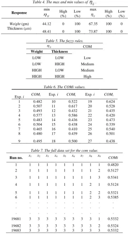
The two quality characteristics are converted into a single response using fuzzy logic. Its input variables are the
ij
values, whereas the COMi values are the output. The minimum and maximum values of
ijfor each quality characteristic are shown in Table 4.25 23 21 19 17 15 13 11 9 7 5 3 1 1700 1680 1660 1640 Obser vation In d iv id u a l V a lu e _ X=1664.6 U C L=1695.07
LC L=1634.13 25 23 21 19 17 15 13 11 9 7 5 3 1 40 30 20 10 0 Obser vation M o v in g R a n g e __ MR=11.46 U C L=37.44
LC L=0 (a) Weight. 25 23 21 19 17 15 13 11 9 7 5 3 1 3450 3300 3150 3000
O bser vation
In di vi du al V al ue _ X=3156 U C L=3405.3
LC L=2906.7 25 23 21 19 17 15 13 11 9 7 5 3 1 300 200 100 0
O bser vation
M ov in g R an ge __ M R=93.8 U C L=306.3
LC L=0
(b) Thickness
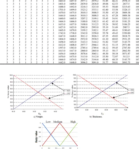
[image:3.595.130.444.342.737.2]The fuzzy logic method is built by setting the inputs and output as shown in Fig. 4. The rules that represent the association between the input variables in the fuzzy model that are represented as
ijfor each quality characteristic and the output are setas shown in Table 5. Then the three fuzzy subsets are assigned to the output value (the COM value) as also shown in Fig. 4.The output of the non-fuzzy value (the COM value) is calculated by using the COG Defuzzification method. The COMivalues obtained from fuzzy logic at eachexperiment are shown in Table 6. The complete data set for the COM value is then generated using RBFNN by setting the orthogonal array as an input matrix and the COM values as an output matrix. The results are displays in Table 7. Finally, the COM averages are calculated at each factor level as shown in Table 8, where the combination of optimal factor levels is x1(1)x2(1)x3(1) x4(2)x5(1) x6(3) x7(3) x8(2)
x9(3), which is identified by selecting the level that
[image:4.595.53.549.204.482.2]maximizes COM average for this factor.
Table 3. The calculated
ij values in the L27 array.Exp. i x1 x2 x3 x4 x5 x6 x7 x8 x9 Wi11 Wi12 Ti21 Ti22
i1
i2Mean Weight
[image:4.595.73.520.273.752.2]Mean Thickness 1 1 1 1 1 1 1 1 1 1 1595.0 1606.0 3180.2 3182.3 46.27 66.62 3181.25 1600.5 2 1 1 2 1 2 2 2 2 2 1673.0 1667.0 3102.1 3104.2 51.90 66.57 3103.13 1670.00 3 1 1 3 1 3 3 3 3 3 1678.0 1675.0 3203.0 3197.0 57.96 57.55 3200.00 1676.5 4 1 2 1 2 1 1 1 2 2 1612.0 1613.0 3170.2 3173.6 67.16 62.51 3171.88 1612.5 5 1 2 2 2 2 2 2 3 3 1647.0 1642.0 3038.8 3042.5 53.35 61.40 3040.63 1644.5 6 1 2 3 2 3 3 3 1 1 1663.0 1657.0 2977.1 2979.2 51.85 66.21 2978.13 1660.00 7 1 3 1 3 1 1 1 3 3 1601.0 1609.0 2839.0 2836.0 49.06 62.53 2837.5 1605.00 8 1 3 2 3 2 2 2 1 1 1688.0 1692.0 3218.3 3213.0 55.53 58.60 3215.63 1690.00 9 1 3 3 3 3 3 3 2 2 1701.0 1699.0 3323.2 3333.1 61.60 53.58 3328.13 1700.00 10 2 1 1 3 1 2 3 1 2 1670.0 1675.0 3010.3 3008.5 53.50 67.28 3009.38 1672.5 11 2 1 2 3 2 3 1 2 3 1644.0 1646.0 3010.3 3008.5 61.31 67.28 3009.38 1645.00 12 2 1 3 3 3 1 2 3 1 1660.0 1665.0 3207.2 3199.1 53.45 54.91 3203.13 1662.50 13 2 2 1 1 1 2 3 2 3 1664.0 1666.0 3180.0 3182.5 61.42 65.10 3181.25 1665.00 14 2 2 2 1 2 3 1 3 1 1633.0 1637.0 3100.0 3112.5 55.24 50.92 3106.25 1635.00 15 2 2 3 1 3 1 2 1 2 1627.0 1623.0 2982.0 2993.0 55.19 51.69 2987.5 1625.00 16 2 3 1 2 1 2 3 3 1 1665.0 1670.0 3199.2 3182.1 53.47 48.41 3190.63 1667.50 17 2 3 2 2 2 3 1 1 2 1742.0 1738.0 3342.0 3358.0 55.78 49.43 3350.00 1740.00 18 2 3 3 2 3 1 2 2 3 1647.0 1648.0 3011.2 3026.3 67.35 49.03 3018.75 1647.50 19 3 1 1 2 1 3 2 1 3 1604.0 1606.0 2932.0 2930.5 61.10 68.83 2931.25 1605.00 20 3 1 2 2 2 1 3 2 1 1658.0 1652.0 3143.3 3144.2 51.82 73.87 3143.75 1655.00 21 3 1 3 2 3 2 1 3 2 1612.0 1608.0 2977.7 2966.1 55.11 51.15 2971.88 1610.00 22 3 2 1 3 1 3 2 2 1 1597.0 1583.0 2785.4 2789.6 44.12 59.45 2787.50 1590.00 23 3 2 2 3 2 1 3 3 2 1613.0 1617.0 2860.0 2865.0 55.13 58.17 2862.50 1615.00 24 3 2 3 3 3 2 1 1 3 1654.0 1646.0 3078.6 3065.1 49.30 50.18 3071.87 1650.00 25 3 3 1 1 1 3 2 3 2 1670.0 1675.0 3113.0 3112.0 53.50 72.87 3112.5 1672.50 26 3 3 2 1 2 1 3 1 3 1666.0 1674.0 3142.9 3144.6 49.40 68.35 3143.75 1670.00 27 3 3 3 1 3 2 1 2 1 1642.0 1648.0 3096.5 3091.0 51.77 58.01 3093.75 1645.00
Table 4. The max and min values of
ij.Response min
ij
High (%) Low (%) max ij High
(%) Low
(%)
Weight (gm) 44.12 0 100 67.35 100 0
Thickness (μm)
48.41 0 100 73.87 100 0
Table 5. The fuzzy rules.
ij
COM
Weight Thickness
LOW LOW Low
LOW HIGH Medium
HIGH LOW Medium
HIGH HIGH High
Table 6. The COMi values.
Exp. i COMi Exp. i COMi Exp. i COMi
1 0.482 10 0.522 19 0.624
2 0.507 11 0.617 20 0.528
3 0.493 12 0.432 21 0.435
4 0.577 13 0.586 22 0.420
5 0.483 14 0.436 23 0.473
6 0.504 15 0.438 24 0.339
7 0.465 16 0.410 25 0.540
8 0.480 17 0.439 26 0.501
9 0.495 18 0.500 27 0.438
[image:5.595.196.398.591.702.2]Table 7. The full data set for the com value.
[image:5.595.185.411.728.786.2]Table 8. The COM averages for the full factorial design.
Table 9. The COM averages for the full factorial design.
Run no. x1 x2 x3 x4 x5 x6 x7 x8 x9 COMi 1 1 1 1 1 1 1 1 1 1 0.4820 2 1 1 1 1 1 1 1 1 2 0.5127
3 1 1 1 1 1 1 1 1 3 0.5341
4 1 1 1 1 1 1 1 2 1 0.5124
5 1 1 1 1 1 1 1 2 2 0.5321 6 1 1 1 1 1 1 1 2 3 0.5385
. . . .
. . . .
. . . .
19681 3 3 3 3 3 3 3 3 1 0.5332
19682 3 3 3 3 3 3 3 3 2 0.5324 19683 3 3 3 3 3 3 3 3 3 0.5332
Factor Level
1 2 3
x1 0.529 0.521 0.527
x2 0.531 0.523 0.526
x3 0.531 0.526 0.525
x4 0.528 0.522 0.524
x5 0.531 0.526 0.525
x6 0.521 0.526 0.529
x7 0.524 0.526 0.529
x8 0.522 0.528 0.526
x9 0.525 0.526 0.531
Response Condition
ˆ
ˆ CˆpkAverage weight Initial 1664.6 10.16 0.41 Online 1669 3.45 1.06
(b) Response Prediction
The weight and thickness averages are predicted at the combination of optimal factor levels
x1(1)x2(1)x3(1)x4(1)x5(1)x6(3)x7(3)x8(2)x9(3) and then the results are
shown in Table 10. It is found that the predicted average weight at the optimal factor levels is 1720.2 ± 17.6 gm, while the predicted average thickness is 3188.515 ± 84 μm. (c) Process adjustment and online sampling
The process parameters are set at the combination of optimal factor settings. During operation, an online sampling is conducted and then the weight and thickness averages are measured. It is found that the injection process exhibits statistical control for both responses. Fig. 5 displays the estimated capability indices for both responses.
III RESULTS AND DİSCUSSİON
The anticipated improvements in both responses are summarized in Table 9, where it is found that:
- For the pipe's weight, the estimated mean,
ˆ, at the combination of initial (optimal) factor settings is equal to 1664.6 (1669), which is close to the target weight value of 1666. The estimated standard deviation,
ˆ, at initial factor settings of 10.16 is reduced significantly to 3.45. As a result, the estimated process capability index, Cˆpk, is significantly improved from 0.41 to 1.06.- For the pipe's thickness, the
ˆ at initial (optimal) factor settings is equal to 3156 (3244.4), which is close to the target weight value of 3200. Moreover, the
ˆ at initial factor settings of 83.11 is reduced significantly to 5.54 using the optimal factor settings. Consequently, the estimated Cˆpk is significantly enhanced from 0.63 to 9.36.- Due to the improvement in individual capability indices, the multiple process capability index, MCpk, index is increased from 0.51 to 3.15, which
indicates that the process becomes highly capable for both quality responses concurrently.
IV CONCLUSİONS
This paper adopted the Process Analytical Technology (PAT) to improve the performance of extrusion process with two main quality responses; pipe's weight and thickness. The main findings of this research is that using Statistical Control Charts to assess process condition at the combination of factor settings demonstrates that the extrusion process is in control while the capability analysis shows poor process performance. Thus, the L27 array is
utilized to provide experimental design, the fuzzy-neural for identifying optimal factor settings and regression models to predict process performance. Confirmation experiments showed that the process means are close to target values of weight and thickness. Moreover, the estimated standard deviation of 10.16 for the pipe's weight at initial settings is
reduced significantly to 3.45 at the optimal factor settings. For the pipe's thickness, the estimated standard deviation at initial settings of 83.11 is significantly reduced to 5.54 using optimal settings. As a result, the estimated process capability index is significantly enhanced from 0.41 to 1.06 for weight and it is significantly increased for thickness from 0.63 to 9.36. The multiple process capability index is increased from 0.51 to 3.15. The main conclusion drawn out of this research is that the gained improvements in extrusion process performance using PAT framework will result in significant savings in quality and production costs.
REFERENCES
[1] A. Al-Refaie and M-H. Li, "Optimizing the performance of plastic injection molding using weighted additive model in goal programming," International Journal of Fuzzy System Applications, vol. 22 (07), pp. 676-689, 2011.
[2] J-C Yu, X-X Chen, T-R Hung, F. Thibault, "Optimization of extrusion blow molding processes using soft computing and Taguchi's method," Journal of Intelligent Manufacturing, vol. 15(5): pp. 625-634, 2004.
[3] A. Al-Refaie, "Optimizing Multiple Quality Responses in the Taguchi Method Using Fuzzy Goal Programming: Modeling and Applications, " International Journal of Intelligent Systems, vol. 30(6): pp. 651-675, 2015.
[4] CDER (Center for Drug Evaluation and Research), "Guidance for Industry: PAT- A Framework for Innovative Pharmaceutical Development, Manufacturing, and Quality Assurance, " US Department of Health and Human Services Food and Drug Administration, 2004.
[5] K. Mandic, B.Delibasic, S.Knezevic, S. Benkovic, " Analysis of the financial parameters of Serbian banks through the application of the fuzzy AHP and TOPSIS methods," Economic Modeling, vol. 43, 30– 37, 2014.
[6] J-H. Sun, Y-C. Fang, B-R. Hsueh, " Combining Taguchi with fuzzy method on extended optimal design of miniature zoom optics with liquid lens," Optik, vol. 123(19) , pp.1768– 1774, 2012.
[7] T. Tsai,―Improving the fine-pitch stencil printing capability using the Taguchi method and Taguchi fuzzy-based model‖, Robotics and Computer-Integrated Manufacturing, vol. 27, pp. 808–817, 2014. [8] A. Marvuglia, A.Messineo, G. Nicolosi, " Coupling a neural network
temperature predictor and a fuzzy logic controller to perform thermal Comfort regulation in an office building," Building and Environment, vol. 72, pp. 287-299, 2014.
[9] S.X. Chen, H.B. Gooi, M.Q. Wang, " Solar radiation forecast based on fuzzy logic and neural networks," Renewable Energy, vol. 60 , pp.195-201, 2013.
[10] Y Mu, G Zhao, X. Wu, " Optimization approach for processing design in the extrusion process of
plastic profile with metal insert, " e-Polymers, 12(1), pp. 353- 366, 2013.