Computing of Mutual Admittance between Two Circumferential Slots on Cylindrical Waveguide

http://www.scirp.org/journal/ojapr ISSN Online: 2329-8413 ISSN Print: 2329-8421

DOI: 10.4236/ojapr.2017.54015 Dec. 21, 2017 188 Open Journal of Antennas and Propagation

Computing of Mutual Admittance between Two

Circumferential Slots on Cylindrical Waveguide

Ali Khayati

1

, Amir Amirabadi

2

, Behnam Rajabi

3 1_{Islamic Azad University Parand Branch, Parand, Iran}

2_{Islamic Azad University South Tehran Branch, Tehran, Iran} 3_{Islamic Azad University Tuyserkan Branch, Tuyserkan, Iran}

Abstract

This paper studies radiation from circumferential slots on cylindrical wave-guide by Poynting’s vector method. It can help us to find mutual admittance between two circumferential slots in an antenna array. The main advantage of Poynting’s vector method is its accurate convergence to compute mutual ad-mittance between two circumferential slots. The importance of this matter will be more salient while we want to compare it with other mutual admit-tances and also use it to optimize an antenna array.

Keywords

Circumferential Slot, Cylindrical Waveguide, Poynting’s Vector, Mutual Admittance

1. Introduction

Electromagnetic radiation from an aperture waveguide is one kind of classical and practical problems which has been considered for several years. Because of cylindrical waveguide and conformal antenna applications, same as aperture waveguide radiation, electromagnetic radiation from slots on cylindrical wave-guide is a prominent problem. To have a better analysis, desired pattern and also to have a proper matching in input, electromagnetic radiation and mutual coupling between slots present an equation to compute mutual admittance be-tween apertures on cylindrical waveguide.

To compute mutual admittance, apart from aperture shape on cylindrical wa-veguide, there are different methods which have been used but generally they are divided into two general categories:

• _{The methods which are based on reciprocity (reaction) theorem that involve}

How to cite this paper: Khayati, A., Ami-rabadi, A. and Rajabi, B. (2017) Computing of Mutual Admittance between Two Cir-cumferential Slots on Cylindrical

Wave-guide. Open Journal of Antennas and

Propagation, 5, 188-199.

https://doi.org/10.4236/ojapr.2017.54015

Received: September 5, 2017 Accepted: December 18, 2017 Published: December 21, 2017

Copyright © 2017 by authors and Scientific Research Publishing Inc. This work is licensed under the Creative Commons Attribution International License (CC BY 4.0).

http://creativecommons.org/licenses/by/4.0/

DOI: 10.4236/ojapr.2017.54015 189 Open Journal of Antennas and Propagation modal solution [1]-[7] and surface ray or GTD-Solutions [8]

• _{The methods which are based on Poynting’s vector [9].}

In modal analysis method we need to have several mode combinations to ob-tain an accurate approach, if the mode numbers aren’t sufficient, analysis accu-racy will be decreased. To have more mode numbers, radius of cylinder must be increased, so this method is not useful for such a problem which the mode numbers are insufficient. If the radius of cylinder be one or two times bigger than wavelength units, surface ray method or GTD-Solution will be helpful. The method which is used in here is based on Poynting’s vector method due to its advantages for circumferential slot array designing.

This method has much more conformity with cylindrical waveguide to reach convergence. The method which is used in here was suggested by Hill [10] to find input impedance for dipole antenna. It also can be used to find mutual im-pedance between axial slots on cylindrical waveguide [11]. So Poynting’s vector method can be indicated such as following relation:

2π _{* 2}

12 * 0 2 1

2 1 1

ˆ sin d d

c n

Y r

V V θ θ ϕ

=

∫ ∫

E ×H ⋅ (1)

Which Y12 is mutual impedance between two slots number 1 and 2, E2 is far electrical radiated field which is emerged from V2 and

* 1

H is far conjugate

magnetic field which is emerged by V1 in (1).

2. Computing Mutual Admittance

Far field radiation from circumferential slots [12] whereas voltage has cosine distribution can be written as follows:

( )

( )

( )

( )

(

( )

)

( )

2 2

2

cos e

cos

e 2

sinc

π sin _{π sin} 2π

i i

jn

n i

jkr i i

i n

i _{i n}

n j

Wk V

E

j r _{n H ka}

ϕ ϕ

θ

α

θ α

θ _{α θ}

− −

∞ =−∞

 

  _{ }

 

=  

 ₋  _{ }

 

∑

(2)

( ) ( )

( )

(

)

( )

(

( )

)

( )

2 2

2

cos e

e 2

cot

π sin _{π sin}

cos sinc

2π

i i

jm

m i

jkr i i

i n

i _{i m}

m mj

V E

r ka _{m H a}

Wk

ϕ ϕ

ϕ

α

α _θ

θ _{α θ}

θ

− −

∞ =−∞

 

 

 

= −

 ₋  ′

 

 

⋅ _{ }

 

∑

(3)

, E

E

Hϕ = _ηθ Hθ = −_ηϕ (4)

where

W

=

3.5 mm

and k 2π

λ

= which λ is wavelength of propagated wave with vacuum dielectric, a is radius of cylinder and Vi is voltage which is

emerged from distributed field on 𝑖𝑖th slot and αi is slot length depending on

degree. In here ri≈ −r z ki cos

( )

θ

and ϕi is offset of 𝑖𝑖′th slot according to x

axis, η is intrinsic impedance of environment and r,θ and φ are spherical

DOI: 10.4236/ojapr.2017.54015 190 Open Journal of Antennas and Propagation ( )2

( )

.

m

H ′ is derivative of second type of Henkel function. In above relations time-dependent function (ej tω ) is neglected. Now, above relations must be con-sidered for finding mutual impedance so according to (1) the result of *

2× 1

E H

can be presented as follows:

2 =E a2θ θˆ +E a2ϕ ϕˆ

E (5)

1=H a1θ θˆ +H a1ϕ ϕˆ

H (6)

(

) (

)

(

)

* *

2 1 2 2 1 1

* *

1

* * 1

2 1 2 1 2 2

ˆ ˆ ˆ ˆ

ˆ_r ˆ_r

E a E a H a H a

E E

E H E H a E E a

θ θ ϕ ϕ θ θ ϕ ϕ

ϕ θ

θ ϕ ϕ θ θ _η ϕ _η

× = + × +

 

= − =_ + _

 

E H

(7)

Integration path C can be shown as Figure 2:

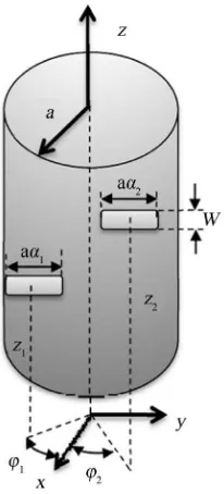
Suppose that in cylindrical coordination system, slot position of I and II are

(

a,

ϕ

2,z2

)

and

(

a,

ϕ

1,z1

)

.

Figure 1. Two circumferential slots on cylindrical

[image:3.595.322.425.294.521.2]

waveguide with their coordination.

[image:3.595.267.483.567.703.2]

DOI: 10.4236/ojapr.2017.54015 191 Open Journal of Antennas and Propagation According to above coordination system, electric and magnetic far field radia-tion is:

( )

( )

( )

( )

(

( )

)

( )

1 1 1 1 1

1 _{2 2}

2 1 ₁ cos e cos e 2 sinc

π sin _{π sin} 2π

jn n jkr n n n j Wk V E

j r _{n H ka}

ϕ ϕ

θ

α

θ α

θ _{α θ}

− − ∞ =−∞     _{ }   =    ₋  _{ }  

∑

(8)

Which r1≈ −r z k1 cos

( )

θ

. For E2ϕ we have:

( ) ( )

( )

(

)

( )

(

( )

)

( )

2 2 2 2 2

2 2 2 2

2 ₁

cos e

e 2

cot

π sin _{π sin}

cos sinc 2π jm m jkr m m m mj V E

r ka _{m H a}

Wk

ϕ ϕ

ϕ

α

α _θ

θ _{α θ}

θ − − ∞ =−∞       = −  ₋  ′     ⋅    

∑

(9)

That r2≈ −r z k2 cos

( )

θ

. Now the result of *

2× 1

E H must be defined, so first of all the term of

1 2

E

E_θ θ

η ∗

must be computed as follow:

( )

( )

(

)

( )

(

( )

)

( )

2 2 2 2 2

2 2 2 2

2 ₂

cos e

cos

e 2

sin

π sin _π sin 2π

jn n jkr n n n j Wk V E c

j r _{n H ka}

ϕ ϕ

θ

α

θ α

θ _{α θ}

− − ∞ =−∞     _{ }   = _{ }  ₋  _{ }  

∑

(10)

( )

( )

( )

( )

( )

(

( )

)

( )

1 1 1 * 1 1

1 _{2 2}

2 * 1 ₁ cos e cos e 2 sinc

π sin _{π sin} 2π

n jn jkr n n n j Wk V E

j r _{n H ka}

ϕ ϕ

θ

α

θ α

θ _{α θ}

− − ∞ ∗ =−∞   − _{   }   =₋    ₋  _{ }  

∑

(11) ( )

( )

(

)

( )

( ) ( ) ( )

(

( )

)

( )

(

( )

)

( )

2 1 2 1 2 1 *

2 1 2 1 1 2

2 2 2 2 2 2

1 2 _{2 1}

2

2 2 *

cos cos

e 2 2

sin _{π π}

cos e e sinc 2π sin sin m n jk r r

m n

jm jn

m n

m n

j

E E V V

r r _{m n}

Wk

H ka H ka

θ θ

ϕ ϕ ϕ ϕ

α

α

α α

η

ηπ

θ

α

α

θ

θ

θ

− − − ∗ ∞ ∞ =−∞ =−∞ − − −             = ⋅  ₋   ₋        ⋅ ⋅    

∑ ∑

(12)

Then for 1

2

E

E_ϕ ϕ

η ∗ we have:

( ) ( )

( )

( )

( )

( )

(

( )

)

( )

1 1 1 * 1 1

1 _{2 2}

2 *

1 ₁

cos e

e 2

cot

π sin _{π sin}

cos sinc 2π n jn jkr n n n n j V E

r ka _{n H ka}

Wk

ϕ ϕ

ϕ

α

α

θ

θ

α

θ

θ

− − ∞ ∗ =−∞   − _{ }   = − ′  ₋      ⋅    

∑

(13)

( ) ( )

( )

(

)

( )

(

( )

)

( )

2 2 2 2 2

2 _{2 2}

2

2 ₂

cos e

e 2

cot

π sin _{π sin}

cos sinc 2π jm m jkr m m m mj V E

r ka _{m H ka}

Wk

ϕ ϕ

ϕ

α

α _θ

θ _{α θ}

DOI: 10.4236/ojapr.2017.54015 192 Open Journal of Antennas and Propagation ( )

( )

(

)

(

( )

)

( ) ( )

( )

(

)

( )

(

( )

)

( )

(

( )

)

( )

2 1 2 1 * 2

1 1 2 2 1

2 ₂ 2

1 2

1 2

2 2 2 2

2 2 *

1 2

2

e

cot

π sin

cos cos e e

2 2

π π sin sin

cos sinc

2π

jk r r

jm jn

m n

m n

m n

E V V

E

r r ka

n m

mnj

n m H ka H ka

Wk

ϕ ϕ

ϕ ϕ ϕ ϕ

α α _θ

η _θ

α α

α α θ θ

θ ∗ − − − − − − ∞ ∞ =−∞ =−∞ =              ₋   ₋        ⋅   ⋅ ′   ′

∑ ∑

(15)

To simplify integral computation, it must be divided in to two parts then compute any part separately and finally the results must be added:

2π _{* 2}

12 ₀ 2 1

2

2π 1 1 2

2 2

0 2

2π _{1 2}

2 0 2

2π 1 2 1 2

2 12 12

1 2 1 1 0 1 1

ˆ sin d d

1

ˆ ˆ sin d d

1

sin d d

1

sin d d

c r r c c c Y nr V V E E

E E a a r

V V

E

E r

V V

E

E r Y Y

V V ϕ θ θ ϕ θ θ ϕ ϕ

θ θ ϕ

θ θ ϕ

η η

θ θ ϕ η

θ θ ϕ η ∗ ∗ ∗ ∗ ∗ ∗ ∗ ∗ = × ⋅   = _ + _     = _{ }     + _ _ = +   ⋅

∫ ∫

∫ ∫

∫ ∫

∫ ∫

E H (16) 1 2π

1 1 2

12 ₀ 2

2

1

sin d d

c

E

Y E r

V V

θ

θ _η θ θ ϕ

∗

∗

 

= _{ }

 

∫ ∫

(17)

2π 1

2 2

12 ₀ 2

2 1 1

sin d d

c

E

Y E r

V V

ϕ

ϕ _η θ θ ϕ

∗

∗

 

= _ _

 

∫ ∫

(18)

In another hand to compute 1 12

Y we have:

( )

( )

(

)

( )

( ) ( ) ( )

(

( )

)

( )

(

( )

)

( )

2 1 2 1 2π

1 1 2

12 ₀ 2

2

2 1

* 2π _{2 1 1 2}

* 0 2 2 2 2 2 2

2 1 1 2 _{2 1}

2

2 *

1

2

1

sin d d

cos cos

e

1 2 2

π sin _{π π}

cos e e sinc 2π sin sin c m n jk r r

c

m n

jm jn

m n

E

Y E r

V V

m n

j V V

V V r r _{m n}

Wk

H ka H ka

θ θ

ϕ ϕ ϕ ϕ

θ θ ϕ η

α α

α α

η θ _{α α}

θ θ θ ∗ − − − _{∞ ∞} =−∞ =−∞ ∗ − − −   = _{ }               =  ₋   ₋        ⋅  

∫ ∫

∑ ∑

∫ ∫

2

sin d d

r θ θ ϕ

 

(19)

According to asymmetry of integration path and term of 1 12

Y , so integration path can be assumed as:

So: ( )

( )

(

)

( )

( ) ( ) ( )

(

( )

)

( )

(

( )

)

( )

2 1 2 1 2π

1 1 2

12 ₀ 2

2

2 1

2π 1 2

2 0 2 2 2 2 2

1 2 _{2 1}

2 2

2 2 *

1

1

sin d d

cos cos

2 e 2 2

π sin _{π π}

cos

e e

sinc sin d

2π

sin sin

c

m n jk r r

c

m n

jm jn

m n

E

Y E r

V V

m n

j

r r _{m n}

Wk

r

H ka H ka

θ θ

ϕ ϕ ϕ ϕ

θ θ ϕ η

α α

α α

η θ _{α α}

DOI: 10.4236/ojapr.2017.54015 193 Open Journal of Antennas and Propagation After substitution of r1 and r2 in (20) and according to even symmetry with respect to φ, integral can be simplify as:

( )( )

( )

(

)

( )

(

)

(

)

(

(

)

)

( )

(

( )

)

( )

(

( )

)

( )

2 1

2 1

cos 2π

1 1 2

12 2 0 2 2 2 2 2

0 0

2 1

2 1 2

2 2 *

cos cos

2 e 2 2

sin

π sin _{π π}

cos cos cos

sinc d d

2π

sin sin

m n

jk z m n

c

m z

n

m n

m n

j Y

m n

m n Wk

H ka H ka

θ ε ε α α

α α _θ

η θ _{α α}

ϕ ϕ ϕ ϕ θ

θ ϕ

θ θ

−

− − ∞ ∞

= =

   

   

   

=

 ₋   ₋ 

   

− −  

⋅  

 

∑∑

∫ ∫

(21)

Which:

1 0

2 0

m

m m

ε =  = ≠ 

if m=n, term of cos

(

m

(

ϕ ϕ

− 2

)

)

cos

(

n

(

ϕ ϕ

− 1

)

)

is an orthogonal function and it has definite values.

So integral can be simplified such as following relations:

( )( )

( )

(

)

( )

(

)

(

)

(

(

)

)

( )

(

( )

)

( )

(

( )

)

( )

2 1

2 1

cos 2π

1 1 2

12 2 0 2 2 2 2 2

0 0

2 1

2 1 2

2 2 *

cos cos

2 e 2 2

sin

π sin _{π π}

cos cos cos

sinc d d

2π

sin sin

jk z n n

c

m n

n

z

n

n n

Y

n n

n n Wk

H ka H ka

θ

α α

ε ε

α α _θ

η θ _{α α}

ϕ ϕ ϕ ϕ θ

θ ϕ

θ θ

− − _{∞ ∞}

= =

  

=

 ₋   ₋ 

   

− −  

⋅  





   

   



∑∑

∫ ∫

(22)

Above relations can be simplified more, if integral be found in term of fol-lowing relations:

( )( )

( )

(

)

( )

(

)

(

)

( )

(

( )

)

( )

2 1

2 1

cos

1 1 2

12 2 2 2 2 2

0

2 1

1 2 2

2

cos cos

4 e 2 2

sin

π sin _{π π}

cos cos

sinc d

2π sin

j

n

z

k z n

c

n

n n

Y

n n

n Wk

H ka

θ ε α α

α α _θ

η θ _{α α}

ϕ ϕ θ

θ θ

− − ∞

=

   

   

   

= ⋅

 ₋   ₋ 

   

−  

⋅ _{ }

 

∑

∫

(23)

The integral can be divided to imaginary and real parts. For real part we have:

( )

π

[ ]

cos , d sin d , 0, , 0

2

z z z

k =k

θ

k = −k

θ θ θ

=_ _→k = k  

So result can be shown as follows:

( )

(

)

( )

(

)

(

)

( )

(

)

2 1

2 1

1 1 2

12 2 2 2 2 2 2

0

2 1

1 2 2

2 0

2 2

cos cos

4 e 2 2

π _{π π}

cos

sinc d

2π

z

jk z n

n z z k

z z

n z

n n

k Y

k k _{n n}

n _Wk

k

H a k k

α α

ε α α

η _{α α}

ϕ ϕ

− − _∞

=

   

   

   

=

−  ₋   ₋ 

   

− _{ }

⋅ _{ }

 

−

∑

∫

(24)

DOI: 10.4236/ojapr.2017.54015 194 Open Journal of Antennas and Propagation

( )

(

( )

( )

)

( )

(

)

(

( )

)

(

( )

)

(

( )

)

cos cos Re Im

cos Re cosh Im sin Re sinh Im

z

k k k j

k

θ

θ

θ

θ

θ

θ

θ

= = +

 

= _ − _

( )

π

( )

[ ]

[

]

Re , Im 0, 0,

2 kz j

θ

=

θ

= ∞ ⇒ = − ∞

It must be mentioned that kz= −jk kz′ ′, z=

[ ]

0,∞ so:

( )

(

)

( )

(

)

(

)

( )

(

)

2 1 2 1

1 1 2

12 0 2 2 2 2 2 2

0

2 1

1 2 2

2 2

2 2

cos cos

4 e 2 2

π _{π π}

cos

sinhc d

2π z

k z z n

n z z z n z n n j k Y

k k _{n n}

n _Wk

k

H a k k

α

α

ε

α α

η

α

α

ϕ ϕ

′ − − _∞ ∞ =             = ′ +  ₋   ₋      −  ′_{ ′} ⋅ _{ }   ′ +

∑

∫

(25) where: sinh 2 sinch 2π 2 z z z Wk Wk Wk ′     ′  ₌     _′  

Same as Y12 we try to find 2 12 Y so:

2π 1

2 2

12 ₀ 2

2 1 1

sin d d

c

E

Y E r

V V

ϕ

ϕ _η θ θ ϕ

∗

∗

 

= _ _

 

∫ ∫

(26)

( )

( )

(

)

(

( )

)

( )

(

)

( ) ( ) ( )

(

( )

)

( )

(

( )

)

( )

2 1 2 1 1 2 * 2

1 1 2 2 1

2 2 2 2 2 2 2

1 2 1 2

2

2 2

cos cos

e 2 2

cot

π sin π π

cos e e sinc 2π sin sin m n jk r r

m n

jm jn

n m

n m

mnj

E V V

E

r r ka n m

Wk

H ka H ka

ϕ ϕ

ϕ ϕ ϕ ϕ

α α

α α _θ

η _{η θ α α}

θ θ θ − ∗ − − ∞ ∞ =−∞ =−∞ − − ∗ −             =    ⋅ ′ ′  − −          

∑ ∑

(27) ( )

( )

(

)

(

( )

)

( ) ( )

( )

(

)

( )

(

( )

)

( )

(

( )

)

( )

2 1 2 1 * 2π 2

2 1 2 2 1

12 _{0 2} 2

2 _{1 2}

1 2

2 2 2 2

2 2 *

1 2 1 2 2 e 1 cot π sin

cos cos e e

2 2

π π sin sin

cos

sinc sin d d

2π

jk r r

c jm jn m n m n m n V V Y

V V _{r r ka}

n m

mnj

n m H ka H ka

Wk

r

ϕ ϕ ϕ ϕ

α α _θ

θ

α α

α α θ θ

θ _{θ θ ϕ}

− − − − − − ∞ ∞ =−∞ =− ∗ ∞ =              ₋   ₋        ⋅ ′ ′ ⋅ _{ }  

∫ ∫

∑ ∑

(28)

( )

( )

(

)

(

( )

)

( )

(

)

( ) ( ) ( )

(

( )

)

( )

(

( )

)

( )

2 1 2 1 1 2 2π 2

2 2 1

12 2 0 2 2 2 2 2

1 2 _{1 2}

2 2

2 * 2

cos cos

e 2 2

cot

π sin π π

cos

e e

sinc sin d d

2π

sin sin

m n jk r r

c m n jm jn n m n m mnj Y

r r _{ka n m}

Wk

r

H ka H ka

ϕ ϕ ϕ ϕ

α α

α α _θ

θ α α

θ

θ θ ϕ

DOI: 10.4236/ojapr.2017.54015 195 Open Journal of Antennas and Propagation ( )( )

( )

(

)

(

( )

)

( )

(

)

( ) ( )

( )

(

( )

)

( )

(

( )

)

( )

2 1

2 1

1 2

cos

2π 2

2 2 1

12 2 0 2 2 2 2 2

1 1

1 2

2 2

2 2

cos cos

2 e 2 2

cot

π sin π π

cos

e e

sinc sin d d

2π

sin sin

m n jk z z

c

m n

jm jn

m n

n m

mnj Y

ka n m

Wk

r

H ka H ka

θ

ϕ ϕ ϕ ϕ

α α

α α _θ

η _{θ α α}

θ

θ θ ϕ

θ ∗ θ

−

− − _{∞ ∞}

= =

− − −

   

   

   

=

 ₋   ₋ 

⋅

   

 

 



′ ′ _

∑∑

∫ ∫

(30)

According to orthogonality property, “m” is equal to “n” so: ( )( )

( )

(

)

(

( )

)

(

)

(

)

(

(

)

)

( )

(

)

( )

(

( )

)

( )

2 1

cos

2π 2

2 2 1

12 2 0 2

2 1 2

2 1

2

2 2 2

2 2

1

1 2

2

4 e

cot

π sin

cos cos cos cos

2 2

π π sin

cos

sinc sin d d

2π

jk z

c

z

n

m

Y

ka

n n

n n n

n n H ka

Wk

θ

α α _θ

η _θ

α α _{ϕ ϕ ϕ ϕ}

α α θ

θ

θ θ ϕ

− −

∞

=

=

    _{− −}

   

   

 ₋   ₋ 

   

 

 

 

⋅

′

⋅

∫ ∫

∑

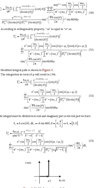
(31)

Modified integral path is shown in Figure 3. The integration in term of φ will result in (34):

( )( )

( )

(

)

(

( )

)

(

)

(

)

( )

(

)

( )

(

( )

)

( )

2 1

cos

2

2 2 1

12 2

2 1 2

1 2

2

2 2 2

2 2

1

1 2

2

8 e

cot

π sin

cos cos cos

2 2

π π sin

cos

sinc sin d d

2π

z

jk z

c

n

m

Y

ka

n n

n n

n n H ka

Wk

θ

α α _θ

η _θ

α α _{ϕ ϕ}

α α θ

θ

θ θ ϕ

− −

∞

=

=

    ₋

   

   

 ₋   ₋ 

   

 

 

 ⋅

 ⋅

′

∫

∑

(32)

The integral must be divided in to real and imaginary part so for real part we have:

( )

π

[ ]

cos , d sin d , 0, , 0

2

z z z

k =k

θ

k = −k

θ θ θ

=_ _→k = k  

( )

(

)

(

)

( )

(

)

( )

(

)

2 1 2

2 2 1

12 2 0 2 2 2 2

2 1 2

1 2

2 2

2 2 2

2 2 2 2

1

1 2

8 e

π

cos cos cos

2 2

sinc d

2π

π π

z

jk z

k _z

z

z

z z

z

z n

m

k Y

a k k k k k

n n

n n

Wk k

n n H a k k

α α η

α α _{ϕ ϕ}

α α

− −

∞

=

=

− −

    ₋

    _{ }

   

 

 

 ₋   ₋  ₋

   

⋅

′

∫

∑

[image:8.595.214.546.68.714.2]

(33)

DOI: 10.4236/ojapr.2017.54015 196 Open Journal of Antennas and Propagation Now imaginary part of path must be computed. At first of hand, path must be modified i.e. for new path we have:

( )

(

( )

( )

)

( )

(

)

(

( )

)

(

( )

)

(

( )

)

cos cos Re Im

cos Re cosh Im sin Re sinh Im

z

k k k j

k j

θ θ θ

θ θ θ θ

= = +

 

= _ − _ (34)

( )

π

( )

[ ]

[

]

Re , Im 0, 0,

2 kz j

θ

=

θ

= ∞ ⇒ = − ∞

Same as above relation: k_z= −jk k_z′ ′, _z=

[ ]

0,∞ so we have: ( )

(

)

(

)

( )

(

)

( )

(

)

2 1 2

2 2 1

12 2 0 2 2 2 2

2 1 2

1 2

2 2

2 2 2

2 2 2 2

1

1 2

8 e

π

cos cos cos

2 2 sinch d 2π π π z k z k z z z z z n n z z j k Y

a k k k k k

n n

n n

Wk k

n n H a k k

α α η

α α _{ϕ ϕ}

α α ′ − − ∞ = ′ = ′ ′ + +     ₋     _{ ′}     _′      −    ′ ⋅ − +     ′

∫

∑

(35)

As a result for totality of 2 12 Y : ( )

(

)

(

)

( )

(

)

( )

(

)

( ) 2 1 2 1 2

2 2 1

12 2 ₀ 2 2 2 2

2 1 2

1 2

2 2

2 2 2

2 2 2 2

1

1 2

2 2 1

2 ₀ 2 2 2 2

2 1

1

8 e

π

cos cos cos

2 2 sinc d 2π π π 8 e π cos 2 z z k z k _z z z z z n n z k z z z z n z z k Y

a k k k k k

n n

n n

Wk k

n n H a k k

j k

a k k k k k

n n

α α η

α α _{ϕ ϕ}

α α α α η α − − ∞ = ′ − − ∞ ∞ = = − −     ₋     _{ }     ⋅ ′ ⋅      −   −  + ′     ′ + ′ ′ + +   

∫

∑

∫

∑

(

(

)

)

( )

(

)

( )

(

)

2 1 2 2 2

2 2 2

2 2 2 2

1 2 cos cos 2 sinch d 2π π π z z n z n n Wk k

n n H a k k

α _{ϕ ϕ}

α α    ₋    _{ ′}    _′      −   − _ ′ + ′    (36)

The totality of Y12 is sum of 1 12

Y and Y122

1 2

12

12 12

Y =Y +Y (37)

12

Y Can be divided in to real and imaginary part:

(

)

(

)

( )

(

)

(

)

( )

(

)

(

)

1 2 2 1 1

12 0 2 2 _{2 2} 2

2 2

0

2 1

1 2 2

2 2 2

2

2 1

2 1

2 0 2 2 2 2

2 2 1 2 1 cos cos cos

4 2 2

π _{π π}

cos sinc d 2π cos 8 π

cos cos co

2 2 n k _z n z z z n z k _z z z z n n n k z G

k k _{n n}

n Wk

k

H a k k

k z k

a k k k k k

n n n z z α α ε α α

η _{α α}

ϕ ϕ α α η α α ∞ = ∞ =         − _{   } = − _{ −   − }     − _{ } ⋅ _{ }   − − + − −             ⋅

∑

∫

∫

∑

(

(

)

)

( )

(

)

( )

(

)

1 2 2 2

2 2 2

2 2 2 2

1 2 s sinc d 2π π π z z n z n Wk k

n n H a k k

DOI: 10.4236/ojapr.2017.54015 197 Open Journal of Antennas and Propagation ( )

(

)

(

)

( )

(

)

( )

(

)

( )

2 1

2 1

2 2 1

12 2 ₀ 2 2 2 2

2 1 2

1 2

2 2

2 2 2

2 2 2 2

1

1 2

2 1

1

2 2

2 0

0

8 e

π

cos cos cos

2 2

sinch d

2π

π π

cos cos

4 e 2

π

z

z

k z

z

z z

z z n

n z

k z n

k

n z

z

z

k B

a k k k k k

n n

n n

Wk k

n n H a k k

n n

k

k k

α α η

α α _{ϕ ϕ}

α α

α α

ε α α

η

′

− −

∞

∞

=

′

− − ∞

=

⋅

′ ′

=

′ ′

+ +

    ₋

    _{ ′}

    _′

 

 

 −   −  + ′

   

 

 

 

+

′ +

∫

∑

∑

∫

( )

(

)

(

)

(

)

( )

(

)

2 2

2 2

1 2

1 2 2

2

2 2 2

2

π π

cos

sinhc d

2π

z z

n z

n n

n Wk

k

H a k k

α α

ϕ ϕ

 

 

 

 ₋   ₋ 

   

−  ′_{ ′}

 

 

′ + ⋅

(

)

(

)

(

)

( )

(

)

(

)

( )

(

)

(

)

(

)

2 1

2 1

1

2 2 2

0 ₀ 2 2 2 2

2 1

1 2 2

2 2 2

2

2 1

2 1

2 2 2 2

2

1 2

2 0

2 1

cos cos

sin

4 2 2

π _{π π}

cos

sinc d

2π

sin 8

π

cos cos cos

2 2

n

k z

n z

z z

n z

k z z

z z

n

n n

k z

k k _{n n}

n _Wk

k

H a k k

k z k

a k k k k

z

k

n n

n n

k

z

α α

ε α α

η _{α α}

ϕ ϕ

α α η

α α

∞

=

∞

=

   

   

− _{   }

−

− _{ −   − }

   

− _{ }

⋅ _{ }

 

−

− +

− −

   

⋅    

∑

∫

∫

∑

(

(

)

)

( )

(

)

( )

(

)

1 2

2 2

2 2 2

2 2 2 2

1 2

sinc d

2π

π π

z z

m z

Wk k

n n H a k k

ϕ ϕ

α α

−

 

 

 

 ₋   ₋  ₋

    ′

(39)

3. Assessment of Parameters Effect on Convergence

The effect of first integral of (39) on total admittance is more than effect of other integrals. Expression of (39) is strongly depended on the term of z2−z1 so that if its value increases, the convergence will not be occurred due to its cosine ex-pression. So according to kz it must be noticed that the term of z2−z1 should be less than wavelength which is propagated in waveguide. Also if the cylinder radius increases so much, it can result in intense reduction of convergence, therefore radius of cylinder must be less than one λ. Susceptance has weak effect on integral totality, so limitation of parameters according to (39) must be men-tioned to enhance convergence.

4. Numerical Results

Now we want to compare analytical results which are came from Poynting’s vector method with simulation results which are yielded by Ansoft HFSS (ver-sion 13) software. For this comparison we consider expan(ver-sion graph of (38) as

( )

12

DOI: 10.4236/ojapr.2017.54015 198 Open Journal of Antennas and Propagation achieved. Cylinder radius is 0.4324λ and slot dimensions as same as each

oth-er are 0.302λ×0.107λ. For this paper, the operation frequency is chosen

9.2GHz and the radius of cylinder 14.1 mm.

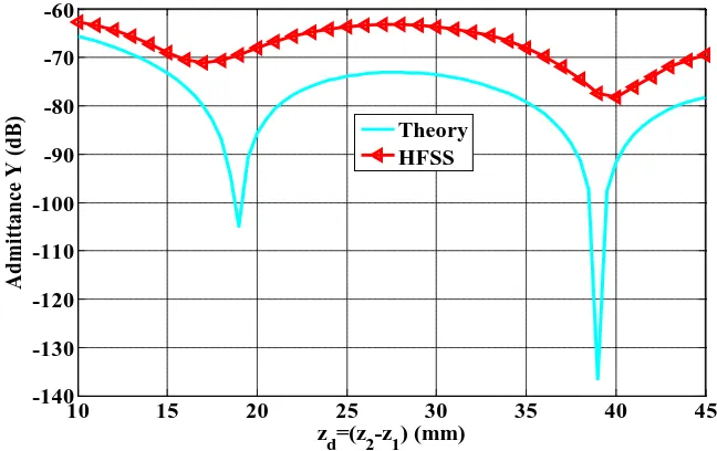
In Figures 1-3 the range of admittance graph for angular offset variations of two slots is between 0 to 400 and distances between slot z2−z1 is constant and it’s equal to 0.54λ.

In Figures 1-4 mutual admittance is zd =z2−z1 and according to wave-length range of distance is between 0.306λ to 1.38λ. The angular offset value

(Figure 5) is ϕd =ϕ ϕ1− 2 =30 deg. And slot aspects as same as each other are

0.302λ×0.107λ. Because of cosine formic, the graph has some depth points.

[image:11.595.208.532.298.502.2]

These points are periodic and summation (in those points), are negligible, therefore logarithmic form of them is consequently insignificant, in the rest of points; graph is similar to simulation result which is yielded by Ansoft HFSS software.

Figure 4. Admittance graph for z2− =z1 0.54λ.

Figure 5. Admittance graph for ϕd=ϕ ϕ1− 2=30 degree.

10 15 20 25 30 35 40 45

-140 -130 -120 -110 -100 -90 -80 -70 -60

z

d=(z2-z1) (mm)

Ad

mi

tt

an

ce

Y (

d

B

)

Theory HFSS

0 5 10 15 20 25 30 35 40

-95 -90 -85 -80 -75 -70

phi_d (Drgree)

Ad

mi

tt

an

c

e

Y (

d

B

)

[image:11.595.209.534.537.705.2]

DOI: 10.4236/ojapr.2017.54015 199 Open Journal of Antennas and Propagation

5. Conclusion

In this paper mutual admittance between two circumferential slots on cylindrical waveguide by extended Poynting’s vector is achieved. Analytical and simulation results are compared the results show good similarity and formulas are pre-sented according to aforesaid limitations on parameters can be useful to find mutual admittance convergence in designing of circumferential slot antennas on cylindrical wave guide.

References

[1] Safavi-Naini, et al. (1976) Calculation of Mutual Admittance between Two Slots on a Cylinder. Attachment A In: Lee, S.W. and Mittra, R., Eds., Study of Mutual Coupling between Two Slots on a Cylinder, Electromagnetic Lab, Department of Electrical Engineering, Urbana.

[2] Golden, et al. (1974) Approximation Techniques for the Mutual Admittance of Slot Antennas on Metallic Cones. IEEE Transactions on Antennas and Propagation, 22, 43-48. https://doi.org/10.1109/TAP.1974.1140727

[3] Stewart, et al. (1971) Mutual Admittance for Axial Rectangular Slots in a Large Conducting Cylinder. IEEE Transactions on Antennas and Propagation, 19, 120-122. https://doi.org/10.1109/TAP.1971.1139875

[4] Oraizi, H., Behbahani, A.K., Noghani, M.T. and Sharafimasouleh, M. (2013) Opti-mum Design of Travelling Rectangular Waveguide Edge Slot Array with Non-Uniform Spacing. Journal of Microwaves, Antennas and Propagation IET, 7, 575-581. https://doi.org/10.1049/iet-map.2012.0438

[5] Masouleh, M.S. and Behbahani, A.K. (2016) Optimum Design of the Array of Cir-cumferential Slots on a Cylindrical Waveguide. AEU-International Journal of Elec-tronics and Communications, 70, 578-583.

https://doi.org/10.1016/j.aeue.2016.01.010

[6] Azarbar, A., Masouleh, M.S. and Behbahani, A.K. (2014) A New Terahertz Micro-strip Rectangular Patch Array Antenna. International Journal of Electromagnetics and Applications, 25-29.

[7] Azarbar, A., Masouleh, M.S., Behbahani, A.K. and Oraizi, H. (2012) Comparison of Different Designs of Cylindrical Printed Quadrifilar Helix Antennas. Computer and Communication Engineering (ICCCE) 2012, Kuala Lumpur, 3-5 July 2012, 18-21.

https://doi.org/10.1109/ICCCE.2012.6271144

[8] Lee, et al. (1982) A Review of GTD Calculation of Mutual Admittance of Slot Con-formal Array. Electromagnetics, 2, 85-127.

https://doi.org/10.1080/02726348208915159

[9] Van Der Pol (1917) On the Wavelengths and Radiation of Loaded Antennas. Pro-ceedings of the Physical Society, 29, 269-289.

[10] Hill (1967) Analytic Determination of Dipole Reactance by Radiation Pattern Inte-gration. Proceedings of the IEEE, 114, 853-858.

[11] Sohtell (1986) Mutual Admittance between Slots on a Cylinder Using the Extended Poynting’s Vector Method. Microwaves, Antennas and Propagation, IEE Proceed-ings H, 133, 238-240. https://doi.org/10.1049/ip-h-2.1986.0042