The simulation of multicomponent ion exchange in fixed bed columns

ION EXCHANGE IN FIXED-BED COLUMNS

A THESIS PRESENTED FOR THE DEGREE OF DOCTOR OF PHILOSOPHY IN CHEMICAL ENGINEERING

UNIVERSITY OF CANTERBURY CHRISTCHURCH; NEW ZEALAND.

by

A. DECHAPUNYA

I would like to thank Dr R.M. Allen, my supervisor,

for his help and guidance throughout this work. Through his

kindness, tolerance and encouragement, the author has brought

the work to a meaningful conclusion.

Many thanks to all the technicians of the Chemical

Engineering Department for their help.

Thanks to Mrs C. McEntee for trying to type everything.

Thanks to Thomas Steele for drawing all the graphs

and proof reading this thesis.

Thanks to Mrs P. Thomas for transforming one copy into many.

The author is grateful to Professor A.M. Kennedy for

arranging a teaching fellowship toward the end of this work.

SUMMARY

1. INTRODUCTION

2. MULTICOMPONENT FIXED-BED ION EXCHANGE EQUATIONS 2.1 The Flux Equations

2.2 The Diffusional Mass Transfer Rate Equations 2.3 The Column Material Balance Equation

2.4 Equilibrium Relations APPENDICES

2A Relationship between the Weight Equivalent Flux Relative to a Fixed Co-ordinate and the Weight Equivalent Flux Relative to Weight Equivalent Average Reference Frame Ve10ci ty.

2B Derivation of Equation 2.3

2C Derivation of Mu1ticomponent Flux Equations from the Nernst-P1anck Equations

2D Derivation of Equations 2.39 and 2.40

3. EVALUATION OF MASS TRANSFER COEFFICIENTS

i

1-1

2-1 2-6 2-14 2-14

3.1 Particle Phase Mass Transfer Coefficients 3-2 3.2 Solution Phase Mass Transfer Coefficients 3-6

3.3 Self-Diffusion Coefficients 3-10

4. NUMERICAL SOLUTION OF MULTICOMPONENT ION EXCHANGE EQUATIONS

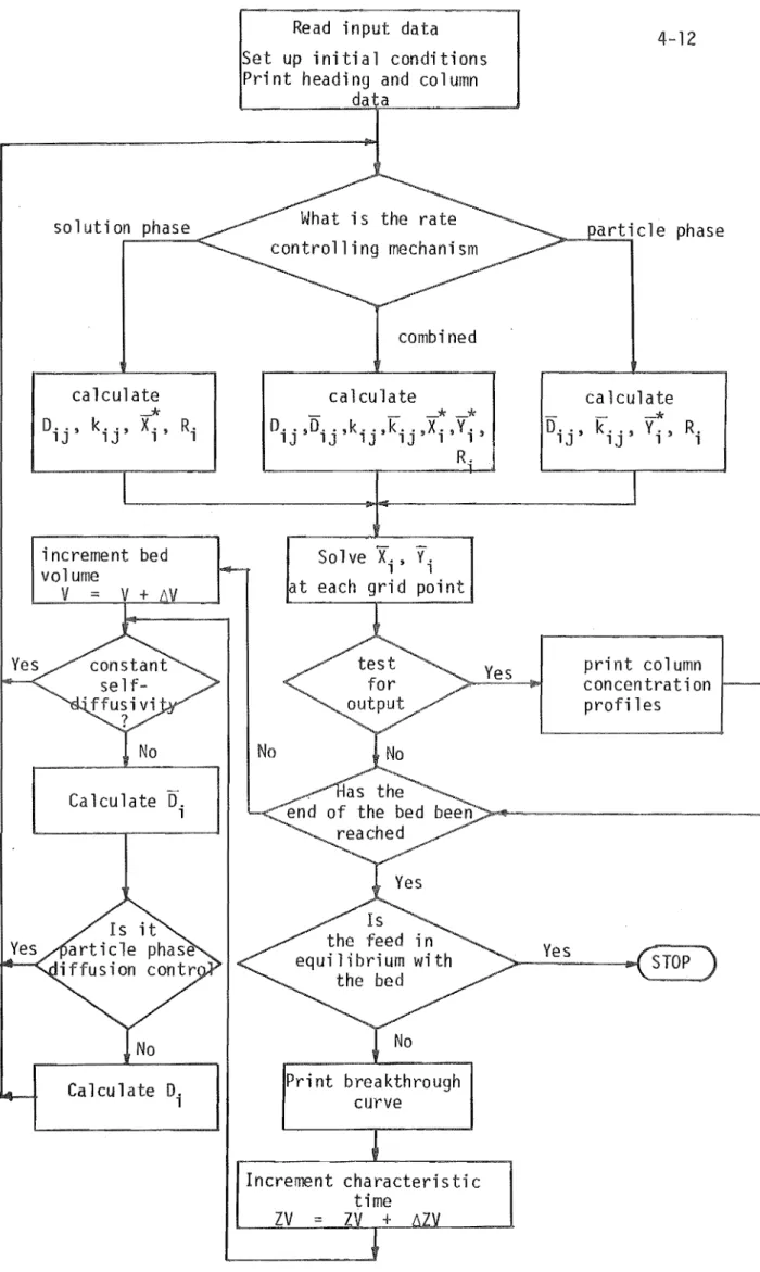
4.1 Equations and Method of Solving 4.2 Initial and Boundary Conditions 4.3 Calculation Procedure

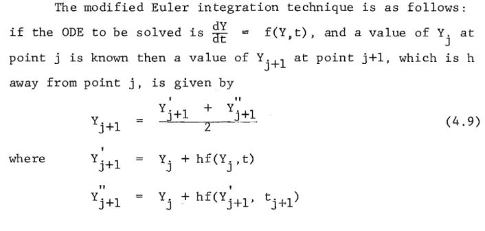
4.4 Numerical Integration Technique 4.5 Combined Rate Mechanism

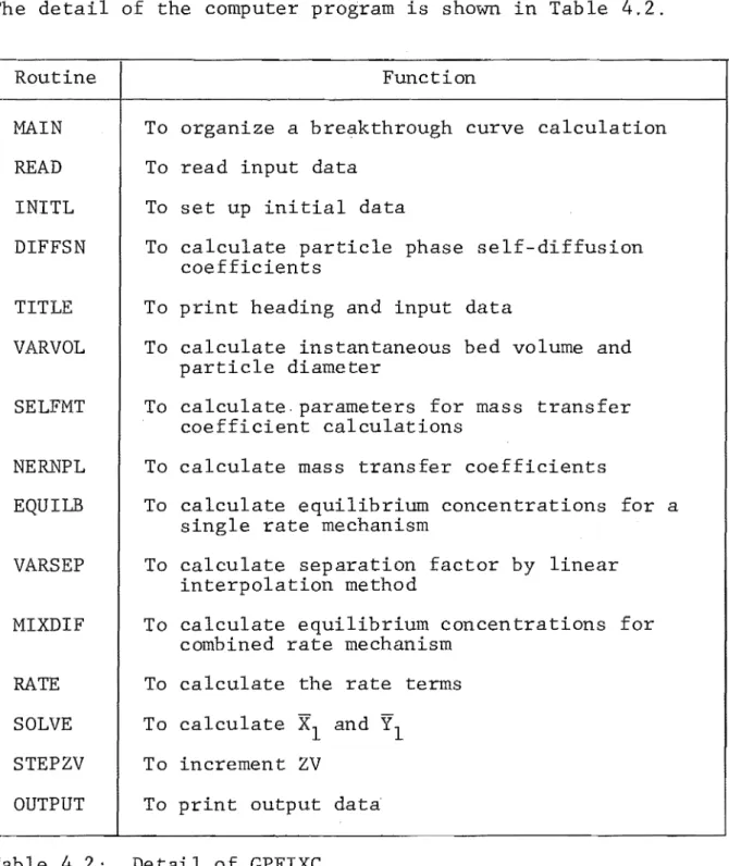
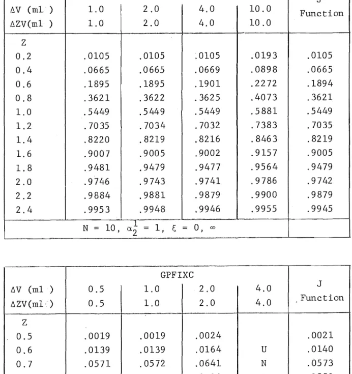
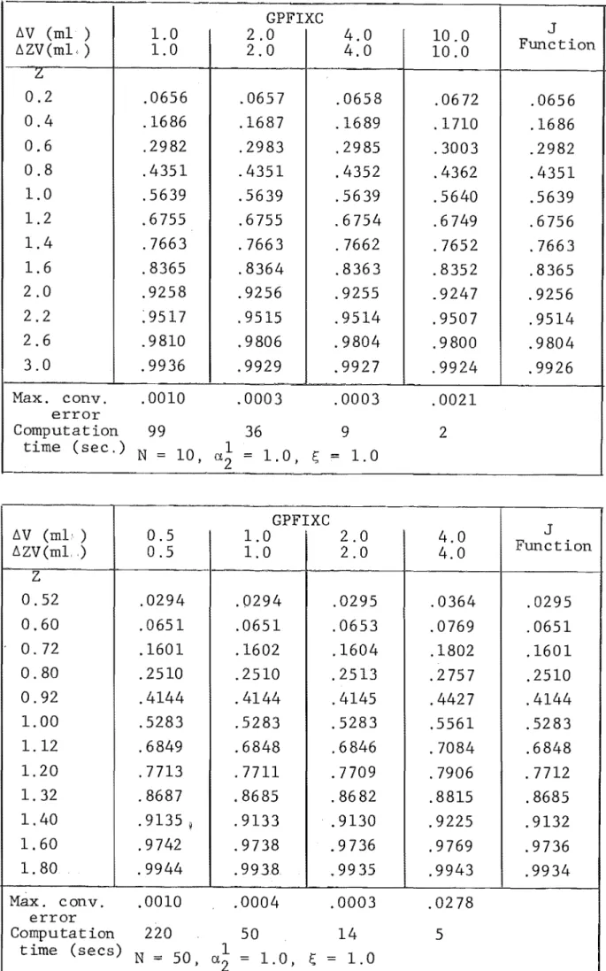
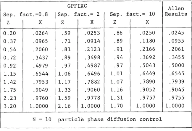
4.6 The Computer Program 4.7 Program Verification

4.9 Comparison with Experimental Results 4.10 Conclusion

APPENDICES

4A User Guide to GPFIXC 4B Program Listing - GPFIXC 4C Sample Output

5. BINARY AND TERNARY ION EXCHANGE EQUILIBRIA 5.1 Introdu~tion

5.2 Experimental Method 5.3 Results

S.4 Discussion APPENDICES

SA Experimental Equilibrium Data SB Capacity Measurement

SC Experimental Procedure in Equilibrium Measurements

SD Error Analysis - Equilibrium Determination 6. COLUMN EXPERIMENTS

6.1 Introduction

6.2 Concentration Measurement

6.3 Effect of Temperature on Column Experiments 6.4 On-Line Monitoring

6.S The Apparatus

APPENDICES

6A Column Experimental Procedure

6B The Nernst Equation and its Use with Ion Selective Electrodes

6C Program Listings for Computing Experimental Breakthrough Curves

6D 6800-Based Data Acquisition System

4-19 4-19

S-l 5-4 5-11 S-16

7.1 Experimental Method

7.2 Results of Binary Experiments 7.3 Results of Ternary Experiments

8. CONCLUSIONS

NOMENCLATURE

REFERENCES

S~RY

A mathematical model based on the Nernst-Planck equations has been developed to describe multicomponent

ion exchange process.

Digital computer programs have been written in FORTRAN IV to solve the equations of the model with the following features:

- mass transfer coefficients are determined from fundamental properties of exchanging ions and ion exchange resins

allowing three exchanging ions for combined mass •

trans resistance or any number for a single phase resistance constant or variable se diffusion coefficients

- constant or variable separation factors

allowing partial column saturation or arbitrary column ini concentration pro les.

To verify the equations of the model a comparison between experimental and predicted breakthrough curves has been made. This involved obtaining independent equilibrium data and measuring column effluent concentration h tories.

Equilibrium studies of K-H, Na-H and K-Na-H systems with Dowex SOW X8 at solution concentration of 0.1 N showed that variable separation factors must be used in the breakthrough curve predictions.

respectively, were recorded by a data logging system consisting

of a Motorola MEK 6800D2 evaluation kit. an Orion 70lA ionalyzer,

a teletype and a IO-bit analog to digital converter.

A comparison of computed results with experimental data

has shown that the model developed can be used to accurately

predict the breakthrough curve behaviour from a multicomponent

CHAPTER 1 INTRODUCTION

There are numerous publications on the science of binary ion exchange operations. The literature was reviewed by Kelly (1966) up to 1966 with the emphasis on experimental work, and by Allen (1973) concentrating on computer simulation work.

Frequently, however, ion exchange operations invoive more than two counter ions. An examination of the literature reveals that references to multicomponent ion exchange in fixed-bed columns are rare. Few experimental breakthrough curves have been published involving more than two counter ions. One

of the reasons the lack of experimental multicomponent breakthrough curves has'; been difficul s in analytical meas-urements. Titrations of samples collected from the columns are tedious and time-consuming. New analytical tools and the low cost of microcomputers allow automat data logging of

continuous column effluent analysis.

The aim of the work is to generate a useful mathematical model of the multicomponent fixed-bed ion exchange process. Experimental results are recorded to verify this model and its numerical solution. This will broadly

involve:-(1) obtaining multicomponent equilibrium data;

(2) obtaining experimental multicomponent breakthrough curves; (3) developing a model or models for multicomponent ion

exchange in fixed-bed columns;

Previous Work on Multicomponent Ion Exchange in Fixed-Bed Columns Dranoff and co-workers (1958, 1961) extended the second order kinetic rate model developed for binary ion exchange to ternary ion exchange. They assumed that equilibrium ratio for any two ions was the same binary and ternary systems. Break-through curve predictions were performed by solving rate,

material balance and equilibrium equations using the method of characteristics. Shallow bed experiments (column diameter 1.5 cm, bed height .25 cm and solution flow rates of 30-116 ml/sq.cm min) were employed to determine rate constants. For each deep bed ternary run (bed height 0.4 5.52 cm) three binary shallow bed runs were prerun to obtain the necessary rate cons.tants for the breakthrough curve prediction of the ternary run. Experimental results showed good agreement between experimental and predicted breakthrough curves. This was to be expected since the exchange was mass transfer controlled and the mass trans constants were experimentally determined. The exchange was said to be mass transfer controlled due to the high flow rates used.

(Samuelson, 1963, recommended flow rates of 3-10 ml/sq.cm min for normal ion exchange operations). Also due to high flow rates, intermediate plateau zones were not developed in one run and were not reached in the others.

A multicomponent ion exchange equilibrium theory (Klein, Tondeur and Vermeulen, 1967) was based on the assumption that at a very low flow-rate mass trans coefficients were high and the ion exchange operation was under equilibrium control, i.e. local equilibrium existed at all points in the bed. Th

of breakthrough curves involved only mass balances and equilibrium

relationships. They showed that the number of plateau zones

equalled, in general, the number of exchanging ions. These

plateau zones were separated by transition zones. The mult

component equilibrium theory is capable of predicting only the

locations of the plateau zones and the transition zones. In

the design of any ion exchange operation, actual dynamics must

be known. l-lork on the dynamic behaviour, the predicting of the

whole breakthrough curves, was carried out by Clazie et al.

(1968) and Omatete (1971).

Clazie applied multicomponent diffusion equations based

on irreversible thermodynamics to ion exchange operations. It

was shown that the multicompon~nt diffusion equation, the

Nernst-Planck equation and the Fick's law equation can be put into the

same

form:-J.

1 = D~. _1J \lX. _J

J. diffusion flux of species i with respect to weight

1

equivalent velocity

Co total solution concentration

D.. multicomponent diffusion coefficient

1J

\lX. driving force for species j.

J

The difference between the three models is the way in which

(1. 1)

Dij was related to basic parameters. The multicomponent rate

equations were obtained by considering the mean concentrations

at a column cross section and applying the linear driving force

approximation to the flux equations. The resulting rate

equations and were solved with appropriate equilibrium data. Predictions of ternary component breakthrough curves involved obtaining mass transfer data from binary column experiments. Ternary equilibrium properties were assumed to be constant and obtained from mass balances on the binary and ternary

breakthrough curves assuming constant pattern conditioruapplied. The Ag-Na-H system with Duolite C-2S porous resin was employed and a total solution concentration of 1.S N was used to ensure particle phase mass transfer control.

Omatete employed the Ag-Na-H system with Dowex SOW X8 non-porous resin. The experiments were carried out at solution concentrations of O.OS N for solution phase diffusion control and 1.S N for particle phase diffusion control.

Both Claz and Omatete experimentally obtained equilibrium and rate parameters binary and ternary breakthrough curves. Even so their agreement between predicted and rimental

breakthrough curves was not good, This may have been because the ion exchange was predominantly under equilibrium control and the equilibrium model used in the breakthrough curve predic tions was not correct. One of the conclusions that the

predicted breakthrough curves were insensitive to the rate terms supported that the exchanging processes were under equilibrium control,

monitored directly by a radioactive tracer technique. Since

the bed contained only one par cle, the amount of exchange

occurring was small and it was assumed that the composition

of the feed solution remained constant. A model (Viswanathan

et al., 1969) was developed to compute the rate of change of

ionic concentration in a resin particle for ternary ion exchange.

The model was a combination of flux eauations based on

irrever-sible thermodynamics and continuity equations. The resulting

rate equations consisted of the time derivatives of counter

ionic concentrations as functions of particle diameter and

particle phase diffusion coefficients. A finite difference

approximation with forward difference formulae was used in

solving the rate equations. The experimental characteristics

were: Sr-Na-Dowex SOW XB, bed diameter 1 cm, total solution

concentration 0.1 N and solution feed flow rate of more than

1500 ml/sq.cm min. High flow rates were employed to ensure

particle phase diffusion control. Satisfactory agreement

between experimental and predicted rate data were obtained in

the favourable equilibrium cases, i.e. when counter ions of

'higher selectivity coe cients replacing other counter ions.

Extensive experimental data under unfavourable equilibrium

conditions for ternary ion exchange in a single particle was

carried out by Bajpai et al. (1974). The Nernst Planck equations were applied instead of those of irreversible thermodynamics.

They pointed out that both principles gave the same equations if

cross phenomenological coefficients were dropped. The systems

unde.r investigation were Mn-Cs-Na, Ba-Mn-Na and Sr ... Mn-Cs with

Dowex SOW

XB.

Agreement between experiment and prediction was

poor for unfavourable equilibrium and this may have been

mechanism. Reasonable improvement was obtained after combined diffusion was introduced into their model. However the

equations used were not presented in the paper.

There appears to be no general analytical solution for IDulticomponent ion exchange. The existing analytical solutions are for special cases, namely constant pattern and those derived from equilibrium theory (Cooney and Strusi, 1972; Bradley and Sweed, 1975).

The science of multicomponent ion exchange in fixed bed columns is far from complete. Current technique needed to be improved and refined as

follows:-(1) The rate terms, Ri, are obtained from binary data; to be able to predict a breakthrough curve of ternary component 1, 2 and 3, binary breakthrough curves of 1 2, 1-3 and 2-3 are needed. Chapter Three considers the possibility of determining the rate terms from fundamental properties of counter ions and ion

exchange resins.

(2) Constant separation factors are employed in breakthrough curve predictions. Binary and ternary equilibrium data will be independently obtained (Chapter 5) .

(3) Combined rate resistances have not been included. Chapter four considers the possibility.

(4) Few ternary breakthrough curves have been presented (Claz 2 curves and Omatete 3 curves). This was due to the method of obtaining experimental breakthrough curves. In this work,

CHAPTER 2

MULTICOMPONENT FIXED-BED ION EXCHANGE EQUATIONS

2.1

The application of irreversible thermodynamics to multi-component diffusion led to a generalized diffusion equation

(Clazie et al., 1968; Viswanathan et al., 1969). For n dependent fluxes and n dependent forces the equations are:

J.

~ =

n E j 1

L ..

vr.

~J J i 1,2, ... n (2.1)

J.

~ weight equivalent flux species i with respect to weight equivalent average reference frame velocity;

L.. weight equivalent phenomonological coefficient for diffusion;

~J

r.

electrochemical potential of species j; J

yr.

gradient of

r.

with respect to distance;

J J

n total number of species in the system, i.e. number of counter ions plus number of co ions plus solvent.

The follmving assumptions are made ding the evaluation of the number of species, n:

(1) The effect of the solvent negligible during ion exchange operations.

(2) The fluxes are considered at the solution-particle interfaces and due to Donnan exclusion principle (Helfferich, 'p.134, 1962) there will be negligible co ions fluxes at the

interfaces.

With these assumptions, n is taken as the number of counter ions.

electrical energies; it can be considered as the driving force

of the ion exchange operation (Helfferich, 1962):

r.

=

].I •

+

Z. f<jJ (2.2)

J J J

in which ].I. ,

J Z. , J f and <jJ are chemical potential, valence, Faraday

constant and electrostatic potential respectively.

The chemical potential of species j can be shown to be

(Appendix 2B) :

].I.

J

t:.

].I. (T I P)

+

RT In X.

J J (2.3)

t:.

where ].I. (T,P), R, T, and X. are ].I. at standard state, universal

J J J

gas constant, absolute temperature and normalized concentration

of species j respectively. Combining Eqn. 2.2 with Eqn. 2.3 gives:

r.

=

].I. t:. (T, P)

+

RT In X.

J J

Upon taking the derivative:

vr.

=

J

+

Z.f\l¢l J

Sqbstituting \lrj in Eqn. 2.1 gives:

J. l

n L:

j 1

L .. RT

lJ [\lX.

X. J J

+

J

+

Z. f<jJ J

(2.4)

The above flux equations are limited in application due to

the difficulties in obtaining L .. values and therefore an approx-lJ

imation will be considered.

The Nernst Planck Approximation

The Nernst Planck equation was derived by Nernst and Planck

in 1889-1890. There are two basic assumptions in the model

1962):-(1) the contribution of e ctrica1 potential is significant; (2) each ionic species interacts with the solvent independently

of the other ions.

The first a basic principle in electrochemistry. The second applies in a dilute solution where the cross coef cients (L .. ;

lJ i ~ j) can be considered negligible in comparison with the main coefficients (Miller; 1966, 1967). Thus Eqn. 2.4 becomes:

defining

where C.

l

J.

l =

L .. RT

I I

X.

l

[VX.

l

+

Z.X.fV¢

l l ]

RT the self diffusion coefficient as:

L .. RT D. == I I

l

is the concentration of species i, Z.X.fV¢ J. == D.C [VX.

+

l l ]

l l 0 l RT

thus

(2.5)

where Co is the weight equivalent total solution phase concentra-tion.

Eqn. 2.5 is applicable to both solution and particle phases. The availability of se -diffusion coefficient data (Chapter 3)

makes the Nernst-P1anck equation practical to implement in ion exchange process calculations.

The electrical potential term in the Nernst-P1anck equation can be eliminated with the following conditions:

(a) Ion exchange is an equi-equiva1ent counter diffusion. Thus, at the solution-particle interface the number of equivalents in the solution and particle phases are constant:

n

E

x·1

1.0

i=l l l .

(2.6A)

n

E

y.,

== 1.0

i=l l l .

where X.

I

and Y.

I

are the normalized concentrations at the inter-1 . 1 .

1 1

face in the solution and particle phases respectively. In the 1m region, the co-ion concentrations would not be expected to be constant because of the possibility of the movement of the ions of different mobilit s (Helfferich, 1962). However, recent investigation by Bajpai et al. (1974) showed that the total

concentration of CIO -ions in the film region can be assumed to be

constant. But in the bulk solution far from the interface, the CO ion concentrations are constant.

(b) The absence of electrical current flow gives the condition that the fluxes of counter ions and cO-ions sum to zero. Due to Donnan exclusion of co-ions, the fluxes of

face are negligib thus

n

L

i=l

n L

i=l

J

.1

1 .

1

I·I

_{1 .}

1

0.0

0.0

ions at the inter

(2.7A)

(2.7B)

where and

J.

I

are the fluxes at the interface in the solution

. 1 .

1 1

and particle phases respectively.

The Nernst-Planck equation for the solution phase with Eqn. 2.6A and Eqn. 2.7A gives (Appendix 2C):

n

J·I

_{1 .} =

1

C L D .• \IX.

I

o. _J 1 1J J .

1

(2.8) j:fi

where the multicomponent solution phase diffusion coefficient D .. is given by:

1J

D .•

1J

Z.X.(D. - D.)

D. [1 + 1 1 J 1 ]

1 n ·

L ~ ~ Dk

1 .

The Nernst-P1anck equation for the particle phase with

Equations 2.6B and 2.7B gives:

n

J·I

Q E

D ..

II _Y·I 1 .

j 1 1J J .

1 1

j#i

(2.10)

where Q is the ion exchange capacity and

D ..

is the mu1ticomponent 1J

particle phase diffusion coefficient given by:

Z.Y.(D.

-

D. )

D .. =

D.

_{[1 +} 1 1 J 1 ] _{(2. 11)}

1J 1 n

E _{Zk Yk}

_1\

k=l

Eqn. 2.8 and Eqn. 2.10 indicate that the flux of species i

is influenced by the concentration gradient of other species. In

other words, there is no concentration gradient of species i

there may still be a flux of species i, provided that other

concentration gradients exist. This fact has been illustrated

experimentally by Cuss1er and Breuer (1972) and Arnold and Toor

(1967) .

The qualitative picture of the Nernst-P1anck model is as

follows. When ions of different mobilities diffuse, an elastic

potential gradient is set up,; this gradient will slow down the

fast ions and speed up the slower ones, i.e. e1ectroneutra1ity

is maintained.

The Nernst-P1anck equations were first applied to the analysis

of particle diffusion in binary ion exchange by He1fferich and

P1esset (1958). Since then, others have applied the Nernst-P1anck

equations to various binary ion exchange systems (Dranoff and

Smith, 1964; Hering and Bliss, 1963; Morig and Rao, 1965; Turner

and co-workers, 1966, 1968, 1970; Kataoka and co-workers, 1968,

Di culties in analytical measurements have hindered the

application of the Nernst-Planck equations to multicomponent

ion exchange in fixed-bed columns (Clazie et al., 1968; Omatete,

1971) .

2.2 The Diffusional Mass Transfer Rate ions

In a fixed bed process, ion exchange takes place because

the feed is not in equilibrium with the bed. The driving force

for the operation is the electrochemical gradient between the

solution phase and the particle phase. For a species i in the

solution phase, its overall concentration gradient is given by

the difference of X. and Y ..

1 1

For strong acid/strong base synthetic ion exchange materials

the transfer mechanism from the solution phase into the particle

phase occurs in three

steps:-(1) Solution phase diffusion

Spec i diffuse from the bulk solution to the

interface.

(2) Adsorption

Species i are adsorbed into the inside of the interface.

(3) Particle phase diffusion

Species i diffuse from the inside of the interface

into the particle.

The adsorption step is usually very fast compared to the

other two, thus its rate does not affect the transfer of species

i into the particle. Consequently, solution phase diffusion and

particle phase diffusion are employed here as a mechanism for

Solution Phase Diffusion

For one particle at a particular cross-section of a fixed-bed column, the rate of diffusion of species i into the particle

is obtained by considering a mass balance between the solution layer around the particle and the particle itself. The rate equation for solution phase diffusion is given by:

ay.

Q

[atl]

V

= -IJ N.

I

l . l

N. weight equivalent flux relative to a fixed co-ordinate

l

N.

I

N. at the solution-particle interface l . l

l

V bed volume t time

(2.12)

The weight equivalent flux relative to a fixed co-ordinate, N., is related to the weight equivalent flux relative to the

l

weight equivalent average frame reference velocity, J., by

l

(Appendix 2A) :

where V

F is the weight equivalent average frame reference velocity. It can be shown that, Appendix 2A, for an ion exchange operation V

F equals zero, thus Eqn. 2.12 becomes:

ay.

Q[at

l

]

V

-IJ J.

I

l .

l

Particle Phase Diffusion

(2.13)

The rate equation for particle phase diffusion is given by:

ay.

Q[at

l

]

V

-IJ J.

I

l .

l

Rate Equations at a Column Cross-Section

(2.14)

exchange column, and therefore the concentrations here are point concentrations. To convert these point concentrations to mean concentrations at a particular cross-section so that they can be coupled with the column material balance equations, the rate equations are integrated over a closed volume

e

bounded by a surface area S. For solution phase diffusion the integration gives:

=

The Gauss theorem gives that

f-(

g.

J. 1 dS

J1S

1 i

where U the unit vector normal to the particle surface. Applying Eqn. 2.16 to Eqn. 2.15 gives:

=

- J.(

g.

J. 1 dS

J1s

1 i

Carrying out the integration gives:

ay.

Q[at 1J8 t =

V

U.J.I

S

- 1 . 1

(2.15)

(2.16)

(2.17)

where 8', Sand

Y.

are bed volume per unit depth, surface area of 1

the particles in the volume per unit depth and mean normalized

concentration at a cross-section of a fixed-bed column respectively. A mass transfer area, A , for ion exchange operation in a

p

fixed-bed column is (Vermeulen, 1958):

where

=

£ and d are void volume per unit bed volume and a particle p

diameter respectively. The relationship between A

A

P =

s

8'

Combining the above equation with Eqn. 2.17 results in

aY.

[at~J

V

For particle phase diffusion Eqn. 2.17 becomes:

ay. "

Q[~J8

V

- D.J.I

- ~ i

s

(2.18)

(2.19)

where 8" is the particle volume per unit depth, related to A p and S by

A

P

and Eqn. 2.19 becomes

ay.

[at~J

V

A

-

Q(l~c)

!I·Ji'i (2.20)

Eqn. 2.18 and Eqn. 2.20 are simplified by substituting J.

~

and J. from Eqn. 2.8 and Eqn. 2.10 respectively:

~

ay. A C n

[at~J p 0 _l:

D .. D. 'VX./ Q

j=l ~J - J .

V ~

(2.21)

jfi

A n

2 l: D .. D. 'VY. ,

V (l-c) j=l ~J ~ J . ~

(2.22)

jfi

Eqn. 2.21 and Eqn. 2.22 can be ther simplified using

the concept the film diffusion theory.

Film Diffusion Approximation

The 1m diffusion theory is based on the following

assumptions:

-(1) The diffusion is a quasi-stationary process; the diffusion

across the film is fast compared with the concentration changes

at the 1m boundaries so that the flux can be computed from

boundary concentrations.

(2) The 1m treated as a planar layer, i.e. the diffusion is one dimensional.

The theory states that all the mass transfer resistances

occur with linear gradients across the film thicknesses (Treybal,

1968). The applications of the film theory to particle phase

diffusion and solution phase diffusion are shown in Figures 2.la

and 2.lb respectively. From Fig. 2.la the varying concentration

gradient is written as:

Y-

.

- y-*.' U.IlY.' =

- 1 .

1 1

(2.23)

1

The negative sign indicates that the unit vector U is normal

outward from the particle surface. Similarly for solution phase

diffusion, Fig. 2.lb,

-T:

u.llx·1

- 1 .

1

(2.24)

1

By combining Eqn. 2.23 with Eqn. 2.22 the particle phase

rate equation is obtained

ay. [at1J

V (1

-n

2::

8)8" j=l j#i

-,,-D ..

(Y. -Y:')

1J J J (2.25)

Also by combining Eqn. 2.24 with Eqn. 2.21 the solution phase

rate equation is obtained

aV. A C n

-i<) [at1J

v

=

~ oQ j=l 2:: D .. 1J (X. J

-

X.' J (2.26) j#i

Defining a multicomponent particle phase mass transfer

coefficient, k .. , and a multicomponent solution phase mass

1J

transfer coe icien t, k

Q A

k ..

=

2 _{£) 6} D •.

~J

e

(1 - ~J

0

(2.27)

A D ..

k .. = E ~J

~J 0 (2.28)

Thus Eqn. 2.25 and Eqn. 2.26 become:

dY.

e

n

-*)

[dt~] = a l.:

k ..

(Y.

Y. (2.29)

V Q j=1 ~J J J

j~i

dY.

e

n .J.

[dt~] =

-

_Q 0 l.: k ..

(X.

X~) (2.30)

V j=1 ~J J J

-*

Y. l. ... x~ l.

X.

Y. l. l. ~---X. U - v

I

I

I

I

I

I

I--0 _ I distance from interface _1-6-t

distance from interface

u.

X. l. Y. l. X, l. ~ X': l. Y. l.

-*

Y. l.

o •

0

(a) (b)

unit vector normal to particle surface normalised solution phase concentration normalised particle phase concentration

mean value of X. at a cross-section of a column 1,

value of

X.

at a particle-solution interface

l.

mean value of y, at a cross-section of a column

l.

value of y, at a particle-solution interface

l.

film thickness, assumed to be constant time average values for the entire duration of mass transfer. It is also

depended on the nature of the flows. The film model works well when

old

and

Kid

are less than unity.

p p

d particle diameter

p

Figure 2.1

Normalized Rate Equations

The normalized column material balance equation, Eqn. 2.37. shows that Y. is a function of V and ZV, i.e. _1.

Y. = f(V, ZV) 1.

where Z is a throughput ratio and is defined as (Vermeulen, 1958): C

Z = Q~ (Ft - VE)

Using the chain rule of partial differentiation on Y. 1.

dY.

=

1.

dY. 1. dt =

ay.

[av1.]dV

+

ZV

aY.

[azt]dZV V

ay.

dV [av 1.] dt

+

ZV

aY.

dZV

[az~] ~

V

By definition ZV

=

=

C F o Q

Combining Eqn. 2.31 with Eqn. 2.32 gives

aY.

[at1.] V

=

(2.31)

(2.32)

(2.33)

Applying Eqn. 2.33 to Eqn. 2.29 and Eqn. 2.30 respectively results

in:

ay.

[az~]

=

V

1 n

- E

F j

j"i

1 n

F

E

j=l j

k ..

(X. - X:';-)

1-J J J

2.3 The Column Material Balance

(2.35 )

The we11known equation describing a material balance of

a species i taken over a cross-section perpendicular to the

direction of the flow in a fixed-bed ion exchange column,

assum-ing that molecular diffusions and 'axial eff,~E;j:::S are negligible, is

given by (Hiester et a1., 1952):

dX.

Q

dY

i

[dV 1-]

+

C[-w-]

+

Vs 0 s V

where Vs is the solution volume.

dX.

£[av1-] s

V

o

(2.36)

By employing the throughput ratio, Z, Eqn. 2.36 can be

shown to be (Allen, 1973):

2.4

dY.

em]

V

+

o

(2.37)

ZV

rium Relation s

A separation factor

a~,

which measures a resin selectively

J

of species i relative to species j at equilibrium, is defined

..I..

-""

--,

i Y. 1-

IX.

1-a. -~'( -;'k~ J _Y.

_IX.

J J

(2.38)

Eqn. 2.38 can be written as (Appendix 2D) i -7(

*

a X.

Y.

= n

1-1- n

aj

..I.. E X'.'

(2.39)

j=l n J n _ .. /<

• f~ a . Y.

- " 1-

1-X. =

1- n _{n -*}

E a. Y.

(2.40)

Equations 2.39 and 2.40 are useful when the diffusion

in a single phase is the controlling mechanism. For example,

-*

when the. particle diffusion is the controlling one, X. equals

l

Xi and one can use Eqn. 2.39 as

-*

a i n X. l

y.

₌

l n

aj

~

_~

APPENDIX 2A

RELATIONSHIP BETWEEN THE WEIGHT EQUIVALENT FLUX RELATIVE TO

A FIXED CO-ORDINATE AND THE WEIGHT EQUIVALENT FLUX RELATIVE

TO WEIGHT AVERAGE REFERENCE FRAME VELOCITY

Let V~ be velocity of species i relative to fixed

co-ordinates. Then V

F the weight equivalent average reference frame velocity is given by:

o n C.V. V E 1. 1.

F i=l

~

C. weight equivalent concentration 1.

Co total concentration

(2A.l)

Now let N. be weight equivalent flux relative to fixed 1.

co-ordinates and J. be weight equivalent flux relative to 1.

weight equivalent average reference frame velocity, therefore

N.

1.

J. =

1.

o C.V.

1. 1.

o

C. (V. - V

F) 1. 1.

The relationship between N. and J. is then 1. 1.

N.

1. = J. 1.

+

C.v'F 1.

(2A.2)

(2A.3)

(2A.4)

An ion exchange operation is an equi-equivalent counter diffusion process i.e. at any time the net fluxes relative to

fixed co-ordinates at the interface are zero so that

n E

1 N.

1.

o

Substituting Ni from Eqn. 2A.2 in the above equation

E

i=l

o

C.V.

~ ~

o

Combining Eqn. 2A.S with Eqn. 2A.l gives

=

o

and Eqn. 2A.4 becomes

N.

=

J.

~ ~

(2A.S)

APPENDIX 2B

DERIVATION OF EQUATION 2.3

The chemical potential of a species i, ~i' is given by

(Robinson and Stokes, 1959)

=

+

RT ln y. M.

~ ~ (2B.l)

o

~i (T,P) chemical potential at a standard state

R

T

P

M.

~

universal gas constant

absolute temperature

pressure

molar concentration

molar activity coefficient

The weight equivalent concentration of species i, C

i , is related to the molar concentration of species i, Mi' by

C.

~ Z .M. ~ ~

where Zi is the valence of species i.

Substituting C. from Eqn. 2B.2 in Eqn. 2B.l gives

~

~

.

~

~

.

~

= ~i o (T, P)

o

~.(T,P)

~

+

"(.C.

RT ln (~)

Z.

~

RT ln Z. + RT ln y. C.

~ ~ ~

(2B.2)

(2B.3)

Since Z. is constant then Eqn. 2B.3 can be written as

~

~

.

~ =

+

RT ln y. ~ C. ~ (2B.4)

The standard state is chosen such that the activity

coefficient approaches unity when the concentration approaches

zero at any temperature and pressure. In Eqn. 2B.4, by definition

state RT ln y. C. equals zero at any temperature and pressure.

~ ~

The concentration in Eqn. 2B.4 can be written in terms of normalized concentration by

=

lJ~(T,P)

~

C

+

RT ln y. C. CO

~ ~

°

lJ. lJ~(T,P)

+

RT ln y. C

+

RT ln X.

~ ~ ~ 0 ~

lJ .

~

=

lJ~(T,P,y.,C

~ ~ 0 )

+

RT In X. ~ (2B.5)

In an ion exchange operation the total number of

equi-valents in anyone phase is constant provided that electrolyte

sorption is negligible and if swelling is also negligible then

Co is constant, Eqn. 2B.S becomes

lJ· _~

+

RT ln X. _~ (2B.6)

For dilute solutions containing homovalent ions, molar

activity coefficients, y., are functions of total solution ionic

~

strength alone (Arpehdix 6B). Since C is constant, then the

o

total ionic strength is also constant, and consequently y. are

~

also constant, Eqn. 2B.6 becomes

APPENDIX 2C

DERIVATION OF MULTI COMPONENT FLUX EQUATIONS FROM THE

tlliRNST-PLANCK EQUATIONS

The Nernst-Planck equation of a counter ion i at the

solution-particle interface is given by (dropping

J.

I.

for clarity),

~ ~

Z.x. f\l ¢ J.

=

-C D.(VX.

+

~ ~T )

~ 0 ~ ~

"I·"

~ from \lX. ~ ~

I.

&

(2C.l)

The absence of electrical current gives the following

conditions, Eqn. 2.7A,

n l: j 1

J.

J

o

Eqn. 2C.2 can be written as

J.

~

+

n l: j 1

j=ri

J.

J

o

Substituting J.

J om Eqn. 2C.l in Eqn. 2C.3 gives

n Z.X.f V¢

J. - l: _{C D. (\lXj} + J J ) 0

~

j 1 0 J RT

j

Solving for f V gives

n

J. l: C D. \lX.

f \l¢ ₌ ~ j=l,j=r i 0 J J

--rtf n

E Z. X. D. Co

j=l J J J jfi

Substituting f V¢/RT in Eqn. 2C.l gives

J.

~ = -C D. o ~ (\lX. ~

Solving for J.

~

+

J. - l: C D.VX. Z.X.[ _{~ ~} ~ _{E . . .} Z X

g

~ JJ)

J J J 0

(2C.2)

(2C.3)

Now

or

or

J.

l ==

J.. =

l

n E X.

j=l J n

E VX.

j=l

VX.

l J

=

o l l

1 n

E

j=l

j:fi

C Z.X.D. o J J J

J J J 0

+

Z.X.D.C l l l 0

E C D.VX. . 0 J J

l

-E C Z.X.D.D.VX.

+

E C D.VX. Z.X.D.

j:f1 0 J J J l l j:fi 0 J J l l l

(2C.S)

= 1.0;

= n E j j:fi

a

VX. J n

E Z.X.D. j=l J J J

Eqn. 2.6A

Substitute VX_i from Eqn. (2C.6) in Eqn. (2C.S)

J. l J. l J. l J. l

=

= n

E C Z.X.D.D.

=1 0 J J J l

n n

n E

j=l

n

+

E C D.VX.Z.X.D.

=1 0 J J l l l

Z.X.D. J J J

n E ( E C Z.X.D.D.)VX.

+

j 1 j=l 0 J J J l J

E C D.Z.X.D.VX. =1 0 J l l l J

n n

E

j=l

Z.X.D.

J J J

E Z.X.D.D.

+

Z.X.D.D.)VX.

=1 J J l J l l l J J

n

n E j 1

E C D.[1.0

. 1 0 l J= j

Z.X.D. J J J

Z.X.(D.-D.) l l J l ]

+

E Z.X.D. VXj

Comparing this equation with Eqn. 1.1

n

J. == C E D •• \IX.

1. _o. 1

J= 1.J J

j j i

the mu1ticomponent diffusion coefficients D .. can be expressed

1.J

in terms of the se1 diffusion coefficients D.

1.

Z.X.(D. - D.)

[1

₊

1. 1. J 1.]

D. . D.

1.J 1. n

E Z.X.D.

APPENDIX 2D

DERIVATION OF EQUATIONS 2.39 AND 2.40

i

A separation factor a _n is given by Eqn ~ . 2 38 . ,

i

a

n (2D.1)

The total solution concentration and the total exchange

capacity can be assumed to be constant, i.e.

n _....

2: V'.'

=

1

i=l l (2D.2)

n _-1(

2: X. 1.0

i=l l (2D.3)

Eqn. 2D.1 can be written as

-'J'(

_,-i .1. Y

V:'

- 1 \ n

= a X. -:r.

l n l _ 1 \

X

(2D.4) n

Summing Eqn. 2D.4 from 1 to n gives .t.

n _ok y" _n n _i - 1 \ .'-E y. -:r. 2: a X.

i=l l - " X 1 n l

(2 D. 5)

n

Combining Eqn. 2D.5 with Eqn. 2D.2 and Eqn. 2D.4 gives

-'-y'." =

l n

E

j=l

-·l~

Similarly for X. it can be shown that

l

n -~~

-•. ;'~ a. y.

l l

X.

::::

l n

n -"Ie

2: a. y.

j 1 J J

(2D.6)

CHAPTER 3

EVALUATION OF MASS TRANSFER COEFFICIENTS

The rate equations which were derIved in section 2.2 are

ay. [at

1J

V

==

C o n

- Q

E' k ..

(X.

-j 1 1J J

C o

Q

j ! i

n E

j=l

j ! i

k.. (Y. 1J J

.'.

X~) for solution phase diffusion J

....

y~) for particle phase diffusion J

k .. and

k ..

are given by Equations 2.27 and 2.28. , 1J 1J

k ..

1J

k ..

1J

Q A

D ..

p 1J C (1-£:)5

o

A D ..

P 1J

o

The multicomponent mass trans coefficients, k .. and k .. ,

1J 1J

are not usually determineq from the above relations due to diffi-culties in obtaining the film thicknesses. A more practical way is to correlate mass transfer coefficients with fundamental

properties using experimental breakthrough curves. The advantage of using an empirical correlation is that i t includes hydrodynamic effects and fundamental properties for which values are available. While mass transfer coefficients are available for isotopic and binary ion exchange there are none presently available for multicomponent ion exchange.

3.1 Particle Phase Mass Transfer Coefficients

To find a particle phase self mass transfer coefficient, k., an isotopic ion exchange is considered. The flux of

~

isotope i at any point inside an ion exchange resin is given by the Nernst lanck equation

J.

~ = -D.Q('ilY. ~ ~

+

Y.Z.f

~ ~

RT

However, since different isotopes are the same counter ion, 'il<P is zero.

(3.1)

The rate of change of concentration in the spherical ion exchange particle is given by the continuity equation

ay. ~

Qat

Equations ay. ~

a t

= -'ilJ.

~

3.1 and 3.2 1 a 2

- [ r

ar

2

r

J.)

~ (3.2)

are combined to give

(3.3) D.

~

For isotopic exchange is constant and Eqn. 3.3 becomes

ay. a2y.

2

~ - [ ~ _{+ (3.4)}

D.

-::--z-~ ar r

Eqn. 3.4 has been solved by many workers (for example Boyd et al,

1947)

under the condition that at t equals zero the surface

concentration changes from Y=0 -"k

-*

i + Yi and remains constant at Yi . Viet) -

~

6

~

1 -4 n2 TI2 t

_=*--~- == 1 - E 2 exp( (3.5)

Y. y~ TIn=ln

~ ~

where Y.(t) is the mean concentration in the particle at time t. ~

Solving for Y.(t) gives ~

Y.

(t) ~

=D _1~

Y.

+

(Y.

~ ~

2 2

6

~

1 -(4n TI Dit)]

Y~) [1 - TI f.., 2."" exp ( 3 .6)

n=l n d2

Eqn'. 3.6 was derived under the condition that the surface

concentration is constant. In ion exchange operations the

surface concentrations are not constant, and the equation has to

be modified before it can be applied to ion exchange operations.

Work of Glueckauf (1955)

Gleuckau,f applied Eqn. 3.6 to a condition in which the

surface concentrations were not constant.

successive integration by parts, that when

of diffusion in a particle is given by

2-4rr D. ..t.

1 - " 2 (Y.

d 1

P

It was shown by

4Dit the rate

- - > 0.1 d2

p

2 2 d2y~~'

315)

~

+. ..

(3. 7) dt

By ignoring the third and higher terms and assuming that

Eqn. 3.7 becomes

dY. 1

dt

(3.8)

60D.

1

7

_p (3.9)

Eqn. 3.9 can be applied at any level in a fixed-bed ion exchange

colunm .

oY.

[ot

1 ]

V

=

60D.

1

7

_p Y. ) 1 (3.10)

While Y_i in Eqn. 3.9 is a mean concentration inside a

particle,

Y

_i in Eqn. 3.10 is the mean concentration at a cross section of a fixed-bed column (Section 2.2).

Work of Hiester and Co-workers (1954, 1956)

Their rate equations were

A DEC .. ~

ay.

[at~]

=

V

A

IT

J~

~ _(Y. - "

8

~ Yi ) for particle phase diffusion (3.12)

ay.

[at~]

V

= _{Y. )}

~ X.)] ~ for reaction

kinetic model (3.13)

D effective solution phase diffusion coefficient

D

effective particle phase diffusion coefficient reaction kinetic mass trans coe cient

A mid-point slope technique was used to determine values of k from experimental breakthrough curves. The procedure can

r

be summarized as follows: (1) from an experimental breakthrough curve, a plot of X vs Z, the slope at mid-point

dx~g.5)

is eval uated; (ii) the value

dX£~.5)

is compared to an analytical plot of

dX£~.5)

vs Nrwhere Nr is the number of transfer units related to reaction kinetic mass transfer coefficient by

k r

F Nr

AIl

F solution flow rate

A column cross section area h bed height

Film thicknesses, 0 and 8, from Equations 3.11 and 3.12 are related to fundamental properties by:

0

Re -m Sc -w

d = a (3.14 )

p

8

b

d == (3.15 )

p

where a, m, wand b are constants, Re and Sc are Reynolds and Schmidt numbers given by

Re =

d Fp

Sc =

where p and ~ are solution phase density and solution phase viscosity respectively.

Substituting 0 and from Equations 3.14 and 3.15 in Equations 3.11 and 3.12 give

v

aY. [at1 ]

V

=

=

A D £ C

P 0 ( -

_x.

a d Re-m Sc-w Q 1

P

(3.17)

(3.18)

(3.19)

The relationship between k , a, b, m and w were shown to be r

BQ

15

6(1-£)))

£C _o D d2 k _r p

a Q IT Re -m S c -w

£ C

D

o

+

b

where B is a correc on term for mixed diffusion control.

(3.20)

Using a number of experimental breakthrough curves from

various workers the constants a, b, m and w were evaluated to

be 0.29, 0.06, 0.5 and 0.5 respectively. Therefore Equations

3.18 and 3.19 become

aY. A D£ C

(ReSc) 0.5 (X. ,', [at1 ]

=

p

0 _{X'.' )}

O.29d

_p Q

-V 1 1

aY. A D ..J.

[at1 ]

=

O.O~

_d (Y:' ₁

-

Y. ) ₁

V _P

Equation 3.22 can be simplified by substituting

6(1-£)/d for A

p

P

aY. [at1 ]

V

100(1 - £)D _{( Y}

*

-- Y.)

d2 i 1

P

(3.2It

(3.22)

(3.22a)

The average value of voidage used in Eqn. 3.20 was 0.4, thus

[ ~,

dl:J V

60 5 (-*

dL

Yi

p

Work of Jury (1967)

Y. )

~ (3.22b)

The Glueckuaf equation, Eqn. 3.9, was verified by an

alternative mathematical approach. In this work Eqn. 3.6 was

solved for variable boundary conditions using a frequency domain

analysis. It was shown that only one assumption, namely

4Dit 1

>

:z

was required in the proof.

1T

Multicomponent Particle Phase Mass Transfer Coefficients

For a single component system Eqn. 2.29 becomes

aY.

[at~]

V

=

C _,~

o '- -" -Q K. (Y.

~ ~ )

Comparing the above equ~tion to Eqn. 3.10 or Eqn. 3.22b

gives

k.

~ (3.23)

The following relation, Eqn. 3.24, will be used to compute

multicomponent particle phase mass transfer coefficients.

k ..

~J =

605 ..

~J

d2 P

(3.24)

where the multicomponent particle phase diffusion coefficient

5 ..

is given by Eqn. 2.11

~J

D .. ~J

z.

Y. (5. - 5.)

D.[l

+ ~ ~ J ~]

~ n

E

z.Y.5.

j=l J J J

3.2 Solution Phase Mass Transfer Coefficients

The flux of isotope i at any point in the 1m layer

between the particle and the bulk solution is given by

The application of the film theory (section 2.2) to Eqn. 3.25 leads to

J·I·

l l -D.C l 0

The rate of change of mean concentration of isotope i in the resin phase is given by the continuity equation

dY.

l

Qat = -A p

u.

~

J.I.

l l

Combining Eqn. 3.27 with Eqn. 3.26 results in

dY.

l

a t

Defining k. as the solution phase self mass transfer

l

coefficien t

A D.

k ~

i 0

Thus, Eqn. 3.28 becomes

dY.

l

a t =

(3.26)

(3.27)

(3.28)

(3.29)

Eqn. 3.29 can be solved under a constant boundary condition and linear equilibrium (Boyd et al., 1947) to give

x.

-

x?

k. C t

l l

= 1 exp[ - l 0 ]

.J ...

-Q

-" _~

x.

-

(3.30)

l l

X. mean normalized concentration at time t

l

-'~

'}C

X.

at the interface at time t

l l

x?

X.

at the interface at time 0

l l

Eqn. 3.30 can be used to correlate k. with fundamental

l

Work of Hiester et al

A relationship between the reaction kinetic mass transfer

coefficient and solution phase and particle phase mass transfer

coefficients was derived for a nonlinear equilibrium. The

mid-point slope technique was used to compute reaction kinetic mass

transfer coefficients from a number of published breakthrough

curves. It was shown that for the solution phase diffusion,

the rate equation is given by:

=

v

6(1 £)D£C o 0.29 d2 Q

p

The term 6(1-£)£D(ReSc)0.5/ 0 . 29 d2 p 3.4482 F£(ReSc)-0.5/_A d .

p Thus

ay.

[at1]

V

3.4482 F£ C

o

=

A d

Q

p

Work of Kataoka et al.

is rearranged to give

(3.31)

The hydraulic radius model was applied to laminar flow in

packed beds by assuming that the voids in the packed beds should

be regarded as a bundle of tubes. The mass transfer between the

particles and the flowing solution becomes the mass transfer

between the inner tube surfaces and the flowing solution. It was

shown that the entrance length, Le, required for a velocity

profile to become fully developed is given by

Le

ci'

P

=

SeRe' _(1-£) (3.32)

where S has a value from 0.022 to 0.029, Re' is Reynolds number

d Fp

given by (l-€)A~ _{and dp '} a distance corresponding to a

spherical diameter based on the hydraulic radius model.

Equation 3.32 indicates that at low Reynolds numbers the

developed at the inlets of imaginary pipes. By solving a

differential mass balance equation for a solute diffusing from

the surface of a tube wall to the flowing solution, a theoretical

liquid phase mass transfer coefficient at high Schmidt number

was shown to be

j

2/3

Sc

=

1 . 85 F Re' - 2

_A£

I

3 (3.33)

Equation 3.33 was tested for ion exchange operations by

comparison with experimental mass transfer coefficients.

Experi-mental data were obtained using isotopic exchange in a single

particle radioactive tracer technique. The relation used for

correlating the experimental results was

X. -

x::

-In (1 - ---::t.;;:---~_1

)

X. -

x<?

1 1

X. -

x::

A

P (3.34)

Plots of In(l _ 1 1

.. J... ~

against t for R-C -C 10.01N and R-Zn-Znl

s s

5C -

X.

1 1

O.OlN showed linear relationships. A plot of j against Rei

(see Eqn. 3.33) on a log-log scale was obtained using experimental

.,'(

data and experimental values of k from the earlier plots. The

plot showed that for Sc > 360 and Re I .< 10 the experimental data

fitted the line drawn by Eqn. 3.33 well.

Multicomponent Solution Phase Mass Transfer Coefficients

For a single component system Eqn. 2.30 becomes

a1.

[at1 ]

V

k. C

_*

=

1 0 (X. _ X.) 1 1

Comparing the above equation with Eqn. 3.31 gives

k. =

1

3.4482 FE(ReSc)-0.5

A d for Hiester relation (3.35)

p

k.

1

1/3

E

1.85(-1-)

-E

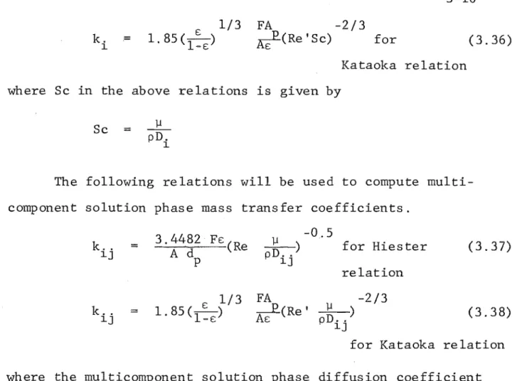
FA -2/3

~(ReISc) for (3.36)

Kataoka relation

where Sc in the above relations is given by

Sc :::: p

The following relations will be used to compute multi

component solution phase mass transfer coe ients.

3.4482 _{FE (Re _]1_)} -0.5

k ..

=

for Hiester

1J A d

p pD .. 1J

(3.37) relation

1/3 FA /3

E _---E.(Re' _]1_)

k .. = _{1. 85(r-)}

1J -E AE pD ..

1J

(3.38)

for Kataoka relation

where the mu1ticomponent solution phase diffusion coefficient

D .. is given by Eqn. 2.9, 1J

D ..

1J = D.[l 1

+

Z.X. (

1 1

Z.X.D. J J J

3.3 Self Diffusion Coefficients

Self diffusion coe cient data, in both solution and

particle phases, are required for mass transfer coefficient

calculations.

Table 3.1 and Table 3.2 show D. and D. respectively for

1 1

a number of ions at various concentrations at 250C.

It is clear from these two tables that self diffusion

coefficients are a function of concentration.

In ion exchange operations, concentration of each ionic

species varies throughout the whole operation and consequently

E1ectroty1e Ion Concen- D. References D?

tration _{2 _1} 1 ₉ 1

(N) ( ms )x10

NaC1 Na+ .000225 1.335 Mills & Godbo1e 1.333

.00102 1.327 (1960)

.00500 1. 319

.0101 1. 312

.0495 1.294

.0970 1.280

LiC1 Li+ 0.2 .962 Anderson & 1.027

0.5 .946 Patterson (1975)

1.0 .919

2.0 .868

NaC1 Na+ 0.2 1.295 " 1.333

0.5 1.279

1.0 1. 234

2.0 1.133

KC1 K+ 0.2 1. 92 II

1. 956

0.5 1. 87

1.0 1. 85

2.0 1. 84

CsC1 Cs+ 0.2 1.952 " 2.054

0.5 1. 947

1.0 1.935

2.0 1. 906

Self diffusion coefficient at infinite dilution is given by the

Nernst equation

D?

=

1

RT At? ₁

(section 6.3)

Counter Concentration Self diffusion

Ion (N) coefficien t References

2 10

( rn , ) x 10

Na+ _{1.0 1.6 Rao and David (1964)}

Na+ _{0.1 2.035 Viswanathan et a1 (1969)}

Sr+ _{0.1 0.190}

Ba+2 _{0.1 0.116}

Na+ _{0.1 2.05 Bajpai et a1 (1974)}

Mn+2 _{0.1 0.222}

Sr +2 0.1 0.195

Ba+2 _{0.1 0.116}

Cs+ _{0.1 3.0}

Na+ _{1.0 1.61 Kataoka, Yoshida and}

Zn+2 _{1.0 0.180 Savada (1974)}

Ba+2 _{1.0 0.0698}

Co+2 _{1.0 0.160}

Na+ _{0.2 1. 57 Graham (1970)}

Cs+ _{0.2 2.41}

algorithm, which estimates self diffusion coefficients in both

the solution and the particle phases at any concentration is

required for breakthrough curve prediction.

Particle Phase Self Diffusion Coefficients

Kataoka and co-workers (1974, 1976) measured sel diffusion

coefficients of H, Li, Na, Cs, Sr, Cu, Ce, Zn, Ba and Co in

many types of ion exchange resin. The isotopic single ion

exchange particle method was used for the experiments . . The

effects of resin diameter, solution concentration, valence,

degree of crosslinking and atomic weight were studied. The

following equations were proposed to estimate self diffusion

coefficients in sulfonated styrene type resin in the range of

degree of cross1inking 3 16%.

D?

~

D.

~

-D?

~

DBa DO

Ba =

v

w H

0.55 exp(-0.174 V-- X Zi)

VW

0.36 exp(-0.348

v

H X)

solution phase self diffusion coe

dilution

v

_HW

bed volume of H-type resin in water

V bed volume in a solution

X degree of crosslinking

Z. valence of species i

~

(3.39)

(3.40)

ient at infinite

When data of VHw/V are not available, they can be estimated

using the following relations. If E is the equivalent weight

of the ion, then for E > 15

VW

H

P = 1.51 .51 Co for 0 < Co < 1.0

P = 1.03 + O.OlC 0.04C 2 for 1 < C < 4

0 0 0

or for E < 15.

VW V w

H ₌ H

V-

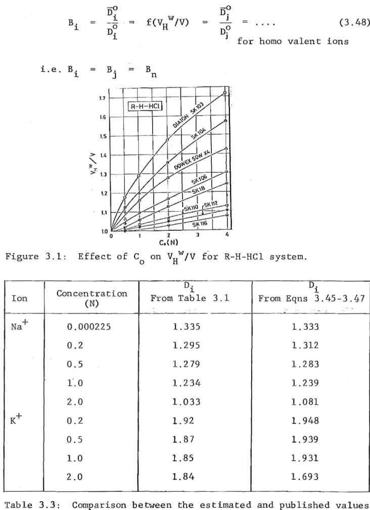
V_H

where the values of VHw/V

H are estimated from Figure 3.1 . . Solution Phase Se If-:diffusion Coefficients

(3.42)

(3.43)

(3.44)

The following relations will be used to determine solution

phase self diffusion coefficients.

Step (l)B. is evaluated at infinite dilution

l

B.

=

l

iY?

l

DC:

l

(3.45 )

::::D

where D. is the particle phase self diffusion coefficient at

l

infinite dilution.

Step (2) assuming that B. is constant for species i, then

l

-0

D.

D.

B. l l (3.46)

l

DC:

D. l l

D.

i. e. D. l (3.47)

l 'i3-:-l

Comparisons between D. computed from Equations 3.45-3.47

l

and D. from literature are shown in Table 3.3. Agreement between

l

experimental and predicted values are good at low concentrations.

Since ion exchange usually involves operation at low

concentra-tions this method of computing solution phase self diffusion

coefficients is acceptable.

In multicomponent ion exchange operations, all counter ions

B.

1 =

D?

₁

n~ = f(VHW/V) 1

i.e, B.

=

B.

=

B

1 J n

1.2

1.1

1-f-,A-/--rY'~-2 c.( N)

=

n?

J for homo va1en t ions

(3.48)

Figure 3.1: Effect of Co on VHw/V for R-H-HC1 system.

D. D.

Concen tration 1 1

Ion _(N) From Table 3.1 From Eqns 3.45-3.47

~

-~~

-~ :

Na+ _{0.000225 1. 335 1.333}

0.2 1.295 1. 312

0.5 1.279 1.283

1'.0 1.234 1.239

2.0 1.033 1.081

K+ _{0.2 1. 92 1. 948}

0.5 1. 87 1.939

1.0 1.85 1. 931

2.0 1.84 1.693

CHAPTER 4

NUMERICAL SOLUTION OF MULTICOMPONENT ION EXCHANGE EQUATIONS

Up to now, no general analytical methods have been

developed to predict breakthrough curves from multicomponent

fixed-bed ion exchange columns. It is possible but unlikely

that there will be an analytical method to solve general

purpose multicomponent ion exchange equations.

Kelly, Allen and Kennedy (1970) stated "there is little to be gained in trying to obtain more precise analytical

descriptions of fixed-bed ion exchange behaviour. Computer

studies allow the considerations of such factors as variable

interdiffusion coefficients, variable separation factor, axial

dispersion, resin volume changes and electrolyte sorption".

This chapter describes the numerical solution of the

rnulticornponent ion exchange equations developed in chapter 2

and chapter 3. The solution is verified against analytical methods and established solutions for binary components.

Comparison is then made with experimental results.

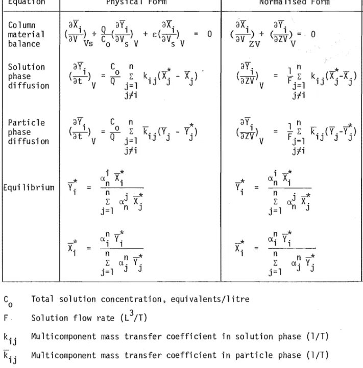
4.1 Equations and Method of Solving

The equations to be solved are presented in Table 4.1 and can be put in the

form:-ay.

(az~)

=

R.

V 1.

i = 1, .... n-l (4.1)

ax.

(av

1.)

=

-R.

ZV 1.