The automatic and quantitative analysis of interferometric and optical fringe data

warwick.ac.uk/lib-publications

A Thesis Submitted for the Degree of PhD at the University of Warwick

Permanent WRAP URL:

http://wrap.warwick.ac.uk/108038/

Copyright and reuse:

This thesis is made available online and is protected by original copyright.

Please scroll down to view the document itself.

Please refer to the repository record for this item for information to help you to cite it.

Our policy information is available from the repository home page.

THE AUTOMATIC AND QUANTITATIVE

ANALYSIS OF INTERFEROMETRIC AND

OPTICAL FRINGE DATA

by

David Peter Towers

Subm itted for the Degree o f

D octor o f Philosophy

in Engineering

at Warwick University

Originally Submitted

7th March 1991,

Revised 28th A pril 1991

Department o f Engineering

Warwick University

A bstract

O ptical interference techniques are used for a wide variety o f industrial mea­ surem ents. U sin g holographic interferom etry or electronic speckle pattern interfer­ om etry, w hole field measurements can be made on diffusely reflecting surfaces to sub-wavelength a ccuracy.

Interference frin ge s are form ed by com paring tw o states of an object. T h e inter­ ference phase co n ta in s information regarding the optical path difference between the tw o object states, a n d is related to the o b je ct deform ation. T h e a utom a tic extraction o f the phase is critica l for optical fringe m etho ds to be applied as a routine to ol. T h e solution to this p ro ble m is the main to p ic o f the thesis.

All stages in th e analysis have been considered : fringe field recording methods, reconstructing th e d a ta into a digital fo rm , and autom atic im age processing algorithm s to solve for th e interference phase.

A new m e th o d fo r reconstructing holographic fringe data has been explored. T h is produced a system w ith considerably reduced sensitivity to environmental changes. A n analysis of th e reconstructed fringe pattern showed th a t m ost errors in the phase measurements are linear. T w o m ethods for error compensation are proposed. T h e op tim u m resolution which can be attained using the m ethod is lambda/90, o r 4 nanometers.

T h e fringe d a ta was digitised using a framestore and solid state C C D camera. T h e image processing followed three distinct stages : filtering the in pu t data, form ing a 'w rapped' phase m a p by either the quasi-heterodyne analysis o r Fourier transform m ethod, and phase unwrapping. T h e prim a ry objective was to form a fully autom atic fringe analysis package, applicable to general fringe data.

A u to m a tic processing has been achieved by making local measurements o f fringe field characteristics. T h e n u m be r of iterations o f an averaging filter is optim ised according to a m easure of the fringe’s signal to noise. In phase unw rapping it has been identified t h a t discontinuities in th e data are m ore likely in regions of high spatial frequency fringes. T h is factor has been incorporated in to a new algorithm where regions o f discontinuous data are isolated according to local variations in the fringe period and d a ta consistency.

The s e m e th o d s have been found to give near o p tim u m results in m any cases. T h e analysis is fully a u tom a ted , and can be performed in a relatively short tim e , «

10

minutes on a S U N 4 processor.

Applications t o static deflections, vib rating objects, axisym m etric flames and tran­ sonic air flows a re presented. S ta tic deflection data from both holographic interfer­ om e try and E S P I is shown.

Contents

1 In troduction 12

1.1 Interference Phase D e t e r m in a t io n ... 14

1.1.1 O p tic a l Heterodyne A n a ly s is ... 19

1.1.2 Q u a si-H e te ro d yn e A n a ly s is ... 20

1.1.3 C a rrie r Fringe M ethods ... 22

1.2 H a rd w a re Requirements for Fringe A n a l y s i s ... 23

1.3 A u to m a te d Evaluation o f General Fringe P a t t e r n s ... 27

1.3.1 P re-P rocessing of Fringe D a t a ... 29

1 .3.2 Frin g e Track in g ... 38

1.3.3 A u to m a tio n of Heterodyne Phase A n a l y s i s ... 46

1 .3.4 A u to m a tic Q u a si-H e te ro d yn e Fringe A n a l y s i s ... 47

1.3.5 A u to m a te d Carrier Fringe Analysis ... 50

1 .3.6 A u to m a tic Phase U n w r a p p i n g ... 55

1.4 S u m m a ry o f Analysis P r o c e d u r e s ...

68

2 In terferom etry, Holography and H olographic Interferom etry 79 2.1 I n t e r f e r o m e t r y ... 79

2 .1.1 L ig h t Sources for Interferom etry and H o lo g r a p h y ... 82

2 .2 H o lo g r a p h y ... - ... 84

2.3 H o lo gra p hic Interferom etry ... 91

2 .3.1 D o u b le Exposure Holographic In te rf e r o m e tr y ... 92

2 .3 .2 T im e -A v e ra g e Holographic In te rfe ro m e try...101

2 .3 .4 S troboscopic Holographic In t e r f e r o m e t r y ... 105

2 .3 .5 C o m b in in g Quasi-H e te ro d yn e Analysis w ith Holographic Inter­ fe ro m e try ...106

2.4 E le ctron ic S peckle Pattern In te rfe ro m e try ... I l l 2.5 A p p lica tio n s o f Holographic Interferom etry and E S P I ...115

2.6 Th e s is F o r m a t ...119

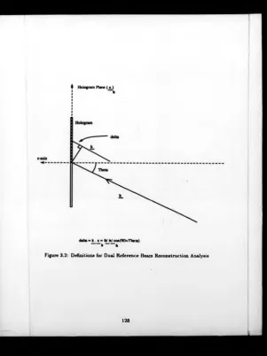
3 Q u asi-H e te rodyn e Analysis o f EYinge P atterns and A u tom atic Im age P rocessin g 124 3.1 D u a l Reference and D ual Reconstruction B eam Holographic Interfer­ o m e try ...124

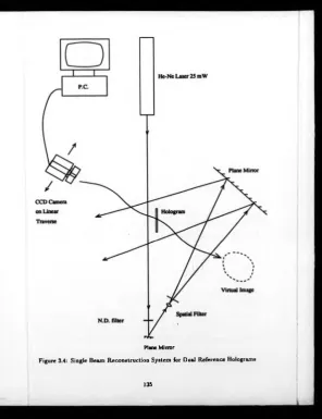
3.2 Single Reconstruction B eam System for Du a l Reference B eam Holog­ ra p hy ... 132

3 .2 .1 A n a lo g y to M oire Fringe P a t t e r n s ...132

3 .2 .2 M athe m a tica l Description o f the Phase Stepping M echanism . 133 3.3 C a p tu re o f Phase Stepped Fringe Fields from th e Single Reconstruc­ tion B e am S y s t e m ... 143

3.4 P re -P ro ce s s in g O f Fringe D a ta ... 153

3.5 A p p lica tio n o f Phase Ste p pin g A lg o rith m s ... 159

3 .5 .1 T h r e e Image Phase Ste p pin g A n a ly s is ... 161

3 .5 .2 F o u r Image Phase S tepping Analysis ... 161

3.6 Phase U n w r a p p i n g ... 163

4 Accu racy an d Resolution Analysis o f H olographic FYinge D ata 170 4.1 Resolution of the Phase Ste p pin g A l g o r i t h m s ...171

4.1.1 Resolution of Phase Stepping Analysis - Dependence on Fringe M o d u la tio n ... 176

4.1.2 Resolution of Phase Stepping Analysis - Dependence on Image N o i s e ... 176

4 .1 .3 Resolution of Phase Ste p pin g Analysis - Dependence on D e­

te c t o r Lin e a rity... 179

4 .1 .4 Resolution of Phase Stepping Analysis - Dependence on the P h a s e S t e p ...182

4.2 A cc u ra c y Achieved in Phase Stepping A n a l y s i s ... 187

4 .2 .1 P ha s e Calculation w ith Th r e e I m a g e s ... 187

4 .2 .2 P ha s e Calculation w ith Fo u r Im a g e s ... 188

4 .3 A cc u ra cy Lim itations for Single Reconstruction B eam Holographic In­ te rfe ro m e try ... 192

4 .3.1 Holographic Recording and Reconstruction Geometries . . . . 192

4 .3 .2 A n a lysis of the Fringe P attern Formed using a Single Recon­ stru ctio n B e a m ... 200

4 .3 .2 .1 Reference Fringe Com pensation - S chem e 1 . . . . 201

4 .3 .2 .2 Reference Fringe C om pensation - S chem e 2 . . . . 206

4 .3 .3 Lin e a rity Assumptions for the Im aging L e n s ... 207

4 .3 .3 .1 Camera Translation to Phase S tep Linearity . . . . 207

4 .3 .3 .2 C am era Translation t o Pixel Shift L in e a rity -...209

4.4 Analysis o f Objects w ith Substantial D e p t h ...215

4 .4 .1 P ha s e Step A n gle Variation w ith O b je ct D e p t h ...215

4 .4 .2 P ix e l Shift Variation w ith O b je c t D e p t h ... 216

4 .5 S u m m a r y ... 217

5 A pplication s o f Dual Reference B e a m Holographic Interferom e­ try and E S P I 222 5.1 T h e Interferom etric Analysis o f S urface Deform ations ... 225

5.1.1 Holographic Analysis o f S ta tic Deflections ...225

5 .1 .1 .1 Reference Fringe C om pensation S chem e 1 ... 236

5 .1 .1 .2 Reference Fringe C om pensation S che m e 2 ... 238

5 .1.2 C om parison o f th e Fourier T ran sfo rm and Phase S te p pin g M e th ­ o d s o f Fringe A n a l y s i s ... 240

5 .1.3 E S P I Analysis of Small S tru ctures in the A u to m o tive Industry 247 5 .1 .3 .1 Phase U n w rapping o f the C ylinder Bore Im age . . . 263 5 .1 .3 .2 Phase Un w rap p ing o f th e C ylinder C h a m b e r Image . 264 5 .1.4 A P u lse d Holographic System fo r Q u a n tita tive Vibration Analysis265 5 .2 T h e Analysis o f Phase Objects using Holographic Interferom etry . . . 275

5 .2.1 A n a lysis o f Burner Flames using Dual Reference B eam Holo­ g ra p h ic In te rfe ro m e try ...280 5 .2 .2 Flow Visualisation in a Large Scale Tran son ic W in d Tu n n e l . . 295

6 Conclusions an d Future Prospects 30 8

7 A ckn ow ledgem en ts 3 1 3

I Characteristics o f Laser Speckle 315

I I Solution o f Q u asi-H e te rodyn e Sim ultaneous Equations 3 1 9

I I I Processing o f H olograph ic Plates 322

I V P ublications 326

List of Figures

1.1 Original Phase D istribution to be R e c o rd e d ... 15

1.2 Intensity D is trib u tio n Corresponding to th e Phase Distribution . . . 16

1 .3 Possible In te rp re tation s of Cosinusoidal Fringe P a t t e r n ... 17

1.4 Developm ents in Personal C o m p u te r Processing P o w e r ... 26

1.5 Example o f an Interferom etric Fringe P a tt e r n ... 30

1 .6 Example o f a Holographic Fringe P a t t e r n ... 31

1.7 Example o f an E S P I Fringe P a t t e r n ... 32

1.8 Am plitude S p e c tra of Interferometric, Holographic, and E S P I Fringe D a t a ... 33

1.9 ES P I Fringe Im a g e After 4 Passes o f a 3*3 Averaging Filter’ . . . . 35

1.10 Comparison o f E S P I Am plitude Spectra Before and A fte r Filtering 36 1.11 Possible D ire c tio n s to Track Fringes ... 38

1 .12 5 * 5 W in d o w f o r Implementing Fringe T r a c k i n g ... 40

1 .13 Five Track e d F rin g e s in an Interference Fringe P a t t e r n ... 41

1 .14 Fo ur C o rre c tly Tra ck e d Fringes in a Filtered Holographic Fringe Im age 42 1 .15 Fo ur Fringes Incorrectly Track e d in a Raw Holographic Fringe Image 43 1 .16 W rapped P ha s e m a p Evaluated by Quasi-H e te ro d yn e Analysis . . . 48

1.17 Sym m etrical S p e c tra of Carrier Fringe Im age R a s t e r ... 50

1 .18 Filtered and Tra n s la te d C arrier Fringe S p e c t r a ... 52

1 .19 Unw rapped p ha se o f Holographic Fringes using a M acy type Algo rithm 60 1 .20 Valid Pixel T e s t for Phase U n w r a p p i n g ... 62

1.21 Holographic W ra p p e d Phase M a p w ith Inconsistent Regions H igh­ lighted in W h i t e ... 63

1.22 Examples o f M in im u m W eight S panning T r e e s ...

66

2 .1 Interferometers d u e to Young, Michelson, and M ach-Z e hn d e r . . . 81 2 .2 T h e G abor system for In-Line Holography ... 87 2 .3 Holographic R e co rd in g System w ith O ff-A x is Reference Beam . . . 89 2 .4 Reconstructed w a ve s from an O ff-A x is H o lo g r a m ... 90 2 .5 Fringe Fun ctio ns fo r Different types o f Holographic Interferom etry . 93 2 .6 Double Pulsed Interferogram of a Vibrational M ode of a T ru m p e t

Bell ... 98 2 .7 Definitions to D e te rm in e the Sensitivity V e c t o r ... 99 2 .8 T i m e Average Interferogram of a C ooling To w e r M o d e l ...103 2 .9 Recording S yste m fo r Dual Reference B eam , Double Exposure Holo­

graphic I n te rf e r o m e tr y ... 107 2 .10 Reconstruction S ys te m for Dual Reference B eam , Double Exposure

Holographic I n t e r f e r o m e t r y ... 108 2.11 Reconstruction S ys te m for Phase Ste p pin g, Real T i m e Holographic

I n te rf e r o m e tr y ... 110 2 .12 O p tica l System f o r Electronic S peckle P attern Interferom etry . . . 112 3.1 Du a l Reference B e a m Holographic Interferom etry w ith Reference

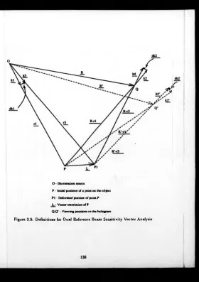
Beam Sources C lo se Together or S e p a ra te d ...127 3 .2 Definitions fo r D u a l Reference B eam Reconstruction Analysis . . . 128 3 .3 Phase Sw eeping M o ire F r i n g e s ... 134 3 .4 Single B eam Reconstruction System for D ual Reference Hologram s 135 3 .5 Definitions for D u a l Reference B e am Sensitivity V e ctor Analysis . . 138 3 .6 Single Beam Reconstruction o f D u a l Reference B eam Hologram

-N o O b je ct D e f o r m a t i o n ... 140 3 .7 Deform ation frin ge s O n a C entrally Loaded D i s c ...141 3 .8 Addition o f Reference Fringes A n d Deform ation Fringes in Single

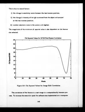
Beam R e c o n s t r u c t i o n ... 142 3 .9 C h i Squared V a lu e s for Image Shift C o rr e la tio n ... 146

3 .10 Definitions t o C alculate Phase Shifting L in e a r i t y ... 147 3.11 Com parison o f C h i Squared distributions for Integer Pixel and 1/4

Pixel Resolution Image T r a n s la t io n ... 151 3 .12 Com parison o f M ethods to Calculate Fringe Field Signal to Noise

R a t i o ...155 3 .13 Com parison o f Measured and Expected Signal to Noise Variations

- Holographic D a t a ...157 3 .14 Com parison o f Measured and Expected Signal to Noise Variations

- E S P I D a t a ...158 3 .15 Sche m atic D ia g ra m of a W rapped Phase M ap S how ing Fringe W ra p ove r

L i n e s ...164 4 .1 Input D a ta t o Phase Stepping A lgo rith m S im u l a t i o n ...172 4 .2 Phase M e a s u re m en t Resolution in Phase Stepping Analysis . . . . 173 4 .3 Phase M e a s u re m en t Errors resulting from a Reduction in Fringe

M odulatio n ...177 4 .4 Phase M ea s u re m e n t Error Variation vs Image N o i s e ... 178 4 .5 Distortion Effe cts o f N on-Linear C am e ra Transfer Function . . . . 180

4.6

Unw rap p e d P hase Distributions S im ulating the Effect of D etector

N o n -Lin e a rity ...181 4 .7 Effect o f P ha s e Step Errors on the Unw rapped Phase D istribution . 182

4.8

Absolute P h a s e Measurement Errors fo r Inaccurate Phase Steps . . 184

4.9

Relative P ha s e Measurement Erro rs for Inaccurate Phase S teps . . 185 4 .1 0 Phase M e a s u re m en t Resolution against Phase S tep M agnitude . . 186 4 .11 C alculated P ha s e Step Distribution - Expected V a lue 120 Degrees . 190 4 .12 C alculated P ha s e Step Distribution - Expected V a lue 80 Degrees . 191 4 .13 R e con struction Arrangem ent in tro d ucin g N otation for Sensitivity

V e ctor E r r o r ... 192 4 .1 4 G eo m e try fo r Spherical Reference B e am Source P o s i t i o n s ... 197 4 .15 G e o m e try fo r Collimated Reference B e a m s ... 199

4 .16 Phase D is trib u tio n Caused by Dual Reference Beam s in th e Holo­ gram Plane ...203 4 .17 Phase Erro r R em aining after Linear C o m p e n s a tio n ... 204 4 .18 Phase S tep V a ria tio n with Trave rse D i s t a n c e ...210 4 .19 Experim ental Arra n ge m en t to Assess Linearity of Pixel Shifting . . 211 4 .20 Pixel Shift V a ria tio n with Trave rse D i s t a n c e ... 214 5.1 Holographic Record in g Arra n ge m en t to Examine th e Deformation

o f a M etal D i s c ... 226 5 .2 G eom etry o f D is c O bject Used for S ta tic Deform ation Tests . . . . 227 5 .3 Filtered and Tra n s la te d Cosinusoidal Fringe Pattern o f the Deformed

D i s c ...230 5.4 W rapped P ha s e M ap of the Deformed D i s c ...231 5.5 Unw rapped P hase Map of the Deformed Disc - Normalised G rey

Scale I m a g e ... 232 5.6 U n w rapped P h a s e Map of the Deformed Disc - Mesh P l o t ... 233 5 .7 Filtered and Tra n s la te d Cosinusoidal Fringe P attern o f the Reference

Beam F r i n g e s ... 234 5 .8 U n w rapped P ha s e Map of th e Reference Beam Fringes - Mesh P lo t 235 5 .9 C om parison o f Reference Fringe Com pensation Schemes Applied to

Holographic Deform ation D a t a ...237 5.10 Cross S ection o f Reference Frin ge Intensity S how ing Distorted Cos­

inusoidal F r i n g e s ... 238 5.11 Cosinusoidal Frin g e Image Suitable for B oth Fourier Tran sfo rm and

Phase S te p p in g A n a lysis ... 241 5.12 W ra p p ed P h a s e M ap formed by F F T M etho d ... 243 5.13 W ra p p e d P h a s e M ap formed by the Phase Stepping M etho d . . . 244 5.14 Unw rap p e d Pha se M ap from the Fourier Tran sfo rm M etho d - N or­

malised G re y Scale I m a g e ... 245 5.15 Un w rap p e d P ha s e M ap from th e Phase S tepping M etho d - Mesh P lot246

5.16 Phase D is trib u tio n Showing the Difference between the Results from

the Phase S te p p in g and Fourier Tran sfo rm T e c h n iq u e s ... 248

5 .17 Fibre O p tic B a se d ES P I S y s t e m ...250

5.18 O p tica l S ystem U se d to Examine C a r Engine Block ...251

5.19 Filtered Cosinusoidal Fringe Image o f the C ylinder B o r e ... 253

5 .20 W ra p p ed Phase M a p for the Cylin d er B o r e ... 254

5.21 U nw rapped P h a s e M ap for the Cylin d er Bore - Normalised G rey Scale I m a g e ...255

5.22 Unw rapped P h a s e M ap for the C ylinder Bore - Mesh P l o t ...256

5 .23 Filtered C osinusoidal Fringe Image o f th e Cylinder Head C ha m be r . 257 5.24 W ra p p ed P hase M a p for the C ylinder Head C ha m be r ... 258

5.25 Unw rapped P ha s e M ap for the C ylin d er Head C ha m b e r - Normalised G re y Scale I m a g e ...259

5.26 U n w rapped P ha s e M ap for the Cylin d er Head C h a m b e r - Mesh P lo t 260 5.27 Progression o f t h e M inim um W e ig h t Spanning Tre e in the Bore Image261 5 .28 Progression o f t h e M inim um W e igh t Spanning T re e in the C ha m be r I m a g e ...262

5.29 High Speed Reference Beam S w itching C o m p o n e n t s ...266

5.30 Holographic A rra n g e m e n t for Vibration A n a l y s i s ...269

5.31 Filtered C osinusoidal Fringe Image o f th e V ib ra tin g S h e e t ...270

5.32 W ra p p ed P hase M a p for the Vib ra tin g S h e e t ... 271

5.33 Unw rapped P h a s e M ap for th e V ib ra tin g Sheet - Normalised G re y Scale I m a g e ...272

5.34 U nw rapped P h a s e M ap for th e V ib ra tin g Sheet - M esh Plot . . . . 273

5.35 Progression o f t h e M inim um W e ig h t Spanning Tre e in the V ib ra tin g Sheet I m a g e ...274

5 .36 Mesh P lo t o f R a m p Corrected Unw rap p e d Phase M a p ...276

5.37 Cross Section o f Original and R am p Corrected U n w rapped Phase M a p s ...277

5.38 O ptical A rra n g e m e n t to Record a Holographic Optical Elem ent from a Diffusing S c r e e n ...282 5.39 Dual Reference Ho lo graphic Recording System for Sm all A xisym

-m etric F l a -m e s ...284 5.40 Filtered Cosinusoidal Fringe Image of th e Lam inar Flam e ...285 5.41 W rapped Phase M a p for the Lam inar F l a m e ...286 5.42 Unw rapped Phase M a p for the Lam inar Flam e - Normalised G rey

Scale I m a g e ...287 5.43 Unw rapped Phase M a p for the Lam inar Flam e - Mesh P lo t . . . . 288 5.44 Mesh Plot o f a La m in a r Flame after Linear Ram p C om pensation . 289 5.45 Use of a M ultich a n n e l H O E to form M ulti-D irectio nal D a ta of a

Phase O b je c t ... 291 5.46 O p tica l S ystem t o A p p ly a 180 degree Phase Change to a Reference

Beam ...292 5.47 C onventional D o u b le Exposure Interferogram of a F l a m e ...293 5.48 Double Exposure Interferogram o f a Flam e with Reference Beam

Phase M o d u l a t i o n ...294 5.49 Schem atic D ra w in g o f the Transonic W in d Tu n n e l at th e Aircraft

Research Associa tio n ...296 5.50 Holographic R e co rd in g System for Tran s on ic Flow in a Te s t C ell . . 297 5.51 Reconstructed Im a g e from an Interferogram of a Sta tic W in g and

E n g i n e ...298 5.52 Holographic R e co rd in g System for Tran son ic External Flow s - W in g

R oot C am era P o s i t i o n ...300 5.53 Holographic R e cord in g System for Tran son ic External Flow s - Side

W a ll C am era P o s i t i o n ... 301 5 .54 Reconstruction fr o m an Interferogram o f Transonic External Flows 303 1.1 S ubjective S pe ck le formed in the Image Plane o f a L e n s ... 316

Chapter 1

Introduction

Interferometric m ethods were established over 100 years ago w ith the w o rk o f N e w ­ ton, Yo un g, Michelson, M ach, an d Zehnder. Standard interferometric m e th o d s were limited to examining specularly reflecting surfaces. T h is restriction was rem oved ap­ proximately 25 years ago by the discovery of holographic interferom etry by Powell and Stetson [1]. Since then m any developm ents have occurred in the techniques used to record and interpret the in form ation contained in an interferogram.

C on cu rre n tly the range o f applications for which th e m ethods offer a solution has grow n. Th e s e applications include :

i) non-destructive testing ( N D T ) [2, 3],

ii) strain analysis due to m echanical or thermal lo ading (4 , 5,

6

], iii) modal analysis o f vibrations [7 ,

8

, 9],

iv ) profile measurement [

10

,

1 1

,

12

],

v ) phase object analysis in clu d ing compressible flows [1 3 , 7 ,1 4 ], te m p e ra tu re measurement [15, 16], a n d plasma diagnostics [1 7 ].

In every case, the required m easurem ent parameter is encoded as a phase cha n ge of the illum ination. W he n tw o (o r m o r e ) light waves are superimposed a frin ge p attern (o r inte rfe rogram ) is produced.

T h e results of an interfe rom e tric experiment are often required by n on-optical specialists. Hence there is a need for methods to analyse a ‘general’ frin ge pattern in order to provide solutions to th e measurement problems listed above. T h e result of any analysis should take th e form of a contiguous phase d istribution. T h i s data may be processed fu rthe r to give the required m easurem ent parameter field assuming some knowledge of the optical system and the object under test. Fo r ro utin e usage, the analysis should be achieved in a fully autom ated m anner and be cost effective. Autom a te d fringe analysis also implies th at an optical system may be used by engineers of different disciplines w ith o u t re-training in a new field.

T h e qu an tity of data co ntained in a fringe field is vast, of the order o f \ G B yte . Furtherm ore, the phase data required is encoded as an intensity m od u lation , usually a cosinusoidal or Bessel fu n ctio n. Im age sensors, such as photodiodes o r cha rg e coupled devices, detect the intensity o f t h e incident light. Hence some means o f data decoding is required to extract the phase data.

Several stages of processing are required to overcom e the problem s o f a utom atic analysis and extraction o f th e phase data.

i) Firstly, optical techniques are required to form th e fringe fields so th a t th e phase data can be decoded.

ii) A sensor is needed to d e te c t the intensity in the fringe field. T h is requires interfacing to an analyser in order to extract the phase inform ation . T h is data m ust then be stored.

iii) T h e complete data analysis system requires automation to ensure cost effectiveness.

T h e current solutions t o these three points are described in sections 1 .1 1.2 1.3. M o s t of the examples in th is work are o f fringe fields w ith a cosinusoidal inten­ sity profile. T h is covers a w id e range of applications : static deform ations, vibration analysis, compressible flows, a n d the measurement of tem perature fields. Vibration analysis, compressible flows, an d the measurement of tem perature fields were

ied using a pulsed laser, w hich also facilitates th e study of transient e ve n ts . T h e occurrence o f Bessel function fringes arises from the study o f vibrations w h e n the exposure tim e for the interferogram is much longer than the tem poral period of the motion [18].

1.1 Interference Phase Determination

Optical techniques have been developed since the first use o f optical interferom eters [19]. Subsequently moire system s, holographic interferom eters, electronic speckle pattern interferometers ( E S P I ) , and shearing systems have been used. In th e case of a static deformation applied to an ob je ct, the fringes formed are cosinusoidal. Th is can be represented by a spatially va ryin g intensity, i ( x , y ) , given by :

• ( * . » ) = • * ( * . » ) • ( 1 + • » (* > » )• CO« ( ¿ ( * . v ) ) ) . ( 1 1 )

where a ( x ,y ) is the local b a ckg rou n d intensity, m ( x , y ) is th e m odulation o f the fringes, and <f> is the phase change t o be measured.

T h e initial analysis o f these frin ge s was by 'fringe co un tin g' (also called th e allo­ cation o f fringe order n u m be rs); e ith e r directly from the fringe field o r a photog ra ph ic record. T h e a m o u n t o f information contained in th e field was reduced by considering only the centres o f the bright (o r d a rk ) bands m aking up the fringe p a tte rn . As a result phase contours were p ro du ce d , and not a contiguous phase map.

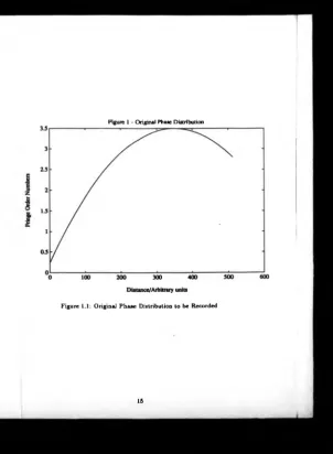
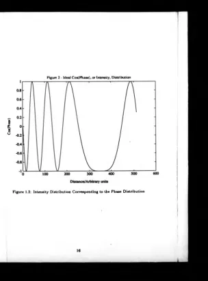
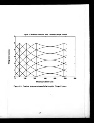
A single cosinusoidal fringe m a p contains insufficient data for a unique solution of the phase to be determ ined. T h i s is due to th e ambiguous nature o f th e fringes. T h e point m ay be illustrated w ith reference to figures 1.1 1.2 1.3. Figu re 1 .1 shows an original phase function to be re corded. A n interferometer produces th e cos o f this function (see figure 1 .2 ). T h is g ra p h may be interpreted in m any different w ays as the phase gradient is not encoded in to the cosinusoidal fringe pattern. H e n c e a t the fringe m axim a, it is unknown w h e th e r to add or subtract 2 xfrom the p hase. T h e possible interpretations of figure 1 .2 are shown in figure 1.3.

Figure 1 - Original Phase Distribution

Figure 1.1: Original Phase Distribution to be Recorded

[image:18.362.27.330.16.429.2]

C

os(

Pha

[image:19.363.37.342.12.424.2]

se)

Figure 2 - Ideal Cos(Phase), or Intensity, Distribution

Figure 1.2: Intensity Distribution Corresponding to the Phase Distribution

[image:20.360.21.325.14.412.2]

Figure 3 - Possible Solutions from Sinusoidal Fringe Pattern

Figure 1.3: Possible Interpretations o f Cosinusoidal Fringe Pattern

Fringe counting relies on human interpretation of the fringe p a tte rn . In this way the sign o f each fringe may be designated from one fringe ce n tre t o the next. T h is process requires a priori information a b o u t the experiment and th e expected result. Even w ith this knowledge of the field, th e re is no guarantee th a t th e correct phase distribution will be achieved. For the successful use o f fringe co u n tin g , the user requires detailed knowledge o f both the o p tic s and the item u n de r test.

A higher measurement resolution could be achieved by interpolation between fringe centres. T h is technique allows m easurem ents to

¿5

of a fringe t o be made in a few cases [20, section 2 .3 ] [19].

1.1.1

Optical Heterodyne Analysis

T h e limitations described 'above were largely rem oved using th e he terodyne and quasi- heterodyne techniques [21, 22, 2 3]. B y o p tic a l heterodyning th e phase information could be directly extracted from the field. T h i s was achieved b y reconstructing the fringe data w ith a beat frequency superposed on the optical frequency. In practice this is achieved by form ing the fringe field w ith tw o waves o f slightly different optical frequency [21]. The s e waves wx and ui

2

m a y be represented by :

» , ( * . » ) = (1 .2 )

and

i » , ( x , » ) = (1 .3 )

where a,-,* =

1 , 2

is th e amplitude o f each w a ve , u » j,i =

1 , 2

is th e optical frequency, = 1 ,2 is the phase o f the wave, and 3? denotes the real p a rt. A photodetector will measure th e tim e-dependent intensity o f th e superposition o f these tw o waves [

2 1

]

■ ( * , » , < ) = |w , + Wil* (1 .4 )

• ( * . » . < ) = » ) + +

2 » i ( i > » ) « > ( * . » ) « * [ ( < « i — » * ) • + * i ( i , l r ) - (1 .5 ) * ( * , » , 0 =

0

|J ( i , l l ) + o ,

1

( l , » ) + 2 o , ( x , K ) a , ( x , v ) c o « [ n i + ^ ( X , » ) ] (1 .6 ) where Q = u>x — u

>2

and ^ ( x , y ) = <t>i(x,y) — f a ( x ,y ) . P ro vid in g th at i l may be resolved by the photodetector, th e o p tic a l interference phase can be measured electronically as th e phase of the beat frequency. O n ce the phase is available rather than a function o f th e phase, the a m b ig u ity in assigning fringe orders is removed. T h u s heterodyning allows a further stage o f th e analysis process t o be automated.

T w o disadvantages remain for he terodyne analysis. Firstly, th e data may only be read o u t in a point-w ise m anner. T h is in h e re n tly limits the processing speed for a

com plete interferogram . Secondly, due to th e trigon o m etric nature o f th e fringes, a given phase difference 6 cannot be distinguished between 6 + m 2ic, m integer. T o overcom e this, a co un t o f the multiples of

2

x is also made as th e data is scanned out. T h i s count can be m ade unambiguously, as opposed to fringe counting, as the interference phase itself is known at all points.

1.1.2

Quasi-Heterodyne Analysis

T h e quasi-heterodyne technique allows the interference phase to be calculated unam ­ biguously as in heterodyne analysis. In this case, the intensity o f a complete fringe field is measured sim ultaneously with a d e te c to r array. Several fringe images are acquired where the phase o f the fringe field is varied either in discrete steps [

22

] or continuously [24]. W h e n discrete steps are added to the frin ge field phase, the m ethod is usually referred to as ‘phase s te p p in g ’ . A num ber o f intensity values are then available for each point in the fringe field. F ro m this data th e interference phase can be calculated in a point-w ise manner.

Conceptually, the m in im u m number of im ages required for quasi-heter.odyne anal­ ysis is tw o [25]. In this case, if a positive phase shift of ^ is applied the direction in which th e fringe maxima m ove indicates w h e th e r th e fringe order n u m b e r is increasing or decreasing. In practice three, four, or five im ages are norm ally used [23,

8

, 26]. W he n three images are used w ith a phase s te p o f 90 degrees, th e th re e images take the fo rm [23] :

where i#(x, y ) is th e intensity at the position (x , y) when the phase step is 0. T h is can be considered as a set o f simultaneous equations w ith un kn o w n s a(x,y), and m (x ,y ). B y algebraically eliminating a (x ,y ) and m (x,y). th e phase may be

* o (* .») = « ( * , » ) . ( 1 + " • ( * ,» ) . CM ( # * , » ) ) ) ,

• »(*.») = •(*.*)•(•-">(*.»)• •“ >(*(*,»))),

•

mo

(* .» ) - o(i,ll).(l -m (x ,* ).co .(* < j:,y ))),

(1 .7 )

(1.8)

(1 .9 )

calculated by :

<t>(x,y) = tan- i f

2

i» o (x , y ) - i

0

( x , y ) - i n o ( x , y )

1

l * o (* » v ) ~ * ie o (* »y) J

(

1

.

10

)

T h e same expression can also be derived as a special case of the analysis by Grievenkamp (27), w here the least squares fit of a sinusoid to th e phase stepped intensity values is con­ sidered.

T h e phase values are evaluated using an a rc tangent fu n ctio n [23]. Hence the results are ‘w ra p p e d ’ into the range — ir to ir. T h e map produced by calculating the phase across th e whole field is called a w ra p p e d phase map. F o r a total variation in optical path difference across an image o f > 2ir, the w ra p p e d phase map will contain discontinuities. T h is makes the w h o le field difficult t o interpret and can cause errors when further com putation m u st b e performed on th e data, for example th e determ ination of strain. T o overcom e th is problem, the phase discontinuities m u st be offset by ‘phase unwrapping’ [22]. In th is process 2 x is added or subtracted from the w rapped phase values every tim e a w ra p o v e r point is reached. W hence, the unwrapped phase map is produced, conta in in g a continuous phase distribution.

T h e variation of background illumination a n d modulation d e p th may also be cal­ culated using :

< o ( * . » ) - N o ( * . y )

<»• (# (* ,»))- « n (# * ,»))

(

1

.

11

)

and

a ( x ,y ) = t

0

( x , y ) — < » ( x , y ) m ( x , y ) c o s ( ^ ( x , y ) ) . ( M

2

) Variations in these tw o parameters allow th e d a ta quality to b e assessed across an image. T h e fringe contrast, o r modulation d e p t h , m ( x , y ) also allows object discon­ tinuities such as holes to be detected a uto m a tica lly [28, 29].

T h e use o f fo ur images in the phase s te p p in g algorithm allow s the phase step to be determ ined w itho ut calibrating the phase shifting m echanism . Alternatively, an increase in th e n u m be r o f images used can in tro d u ce a degree o f redundancy in the

solution w hich in tu rn minimises the errors in the calculated phase (if there exists errors in the in pu t param eters). For exam p le, Hariharan proposed using five images w ith a phase step of 90 degrees to m inim ise measurement erro rs due to inaccurate phase steps [2 6 ].

W ith th e curre n t com m ercial availability o f detector arrays and image digitisers, this m ethod offers rapid data acquisition a n d d ire ct co m pu te r analysis.

1.1.3 Carrier Fringe M ethods

Fringe order am biguities can also be re m o ve d by the addition o f ‘carrier fringes'. In this technique, a linear phase variation is a d d e d to the fringe field as a function of image co -o rdinate. T h is can be achieved in p ra ctice by tiltin g on e o f the mirrors in an interferom eter, thereby givin g a ‘tilted w a v e fr o n t'. T h e intensity in the fringe pattern m ay then be represented by :

»(*,

y) =

a ( x ,y ) .( l + m ( * ,y ) . cos (2w/0* + ¿ ( x ,y ) ) ) , (1 1 3 )

w here /„ is the spatial carrier frequency a ssum ed to be in th e x direction. T h e carrier frequency m u st be sufficiently high so as t o p ro du ce m onotonically increasing fringe order num bers. W h e n this is achieved, th e fie ld can also be described as a finite fringe field, and is characterised by th e absence o f a n y closed lo op fringes. An exam ple of such a field is given in figure 1.5 (contained in section 1 .3 .1 ), w hich was produced by a classical specular interferom eter.

A finite fringe field can be processed b y fringe co un tin g w ith o u t am biguity as th e fringe orders are known to increase m on o to n ica lly in th e direction of th e tilted wavefront. T h e phase data obtained re presents the required measurement param eter added to th e phase of th e tilted w avefront. T h e phase change due to the tilt m u st therefore be calculated and subtracted fr o m t h e original phase information obtained. T h e required param eter m a y then be calcu late d from the resulting phase distribution. T h e usefulness of carrier fringe m e tho d s in interferom etry w a s not fully realised until electronic imaging hardw are and m ore pow erful co m pu te r systems became

able 1.3.5.

1.2 Hardware Requirements for Fringe Analysis

T h e most obvious means to handle large q u an titie s o f information whilst allowing flexi­ ble means o f data processing is to utilise c o m p u te r technology. C om p u te r technology has developed rapidly over the past

20

years and w ith ever-increasing processing power it has enabled the practical im p le m e nta tion of m any o f the optical techniques described above. T h e general requ ire m en ts o f a com puter system to perform fringe analysis are listed below.

i ) C om putational power. T h is is lim ite d by the processing speed o f the microprocessor.

ii) T h e facility to run high level c o m p u te r languages hence allowing flexible user programing.

iii) Large data storage space.

iv ) T h e facility to interface image digitisers, and other devices, to computers thereby form ing an integrated s yste m fo r industrial use.

v ) Rapid data transfer from the s to ra ge devices and co m pu te r interfaces.

v i) A suitable means to o u tpu t th e d a ta .

v ii) Portability, for on-site industrial inspection and analysis.

T h e requirements for each o f these ite m s is continually g row in g due to th e industrial need to evaluate more complex problem s.

T o take advantage o f flexible c o m p u te r analysis, the data m ust first be interfaced to the co m pu te r system. T h is involves t w o components : a sensor to detect the intensity in the fringe field, and a digitiser t o convert the o u tp u t o f the sensor in to a digital fo rm .

Initially, com puters were used in c o n ju n c tio n w ith a digitising tablet to allow th e e n try o f fringe m axima or minim a from a p hotog ra ph . In this case, the sensor was the hum an eye and discrete x , y c o -o rd in a te pairs were in pu t to the com puter. T h e data was detected and processed in a seq u e n tia l manner, thereby limiting the processing speed. S om e increase in the p ro cessing rate was achieved by replacing the hum an eye w ith a photodiode and co m pu te r in te rfa c e [15]. T h e co m p u te r utilised the detected intensity to scan th e diode along frin g e m axim a or m in im a . The s e m ethods o f acquiring digital fringe information were t im e consum ing and o n ly provided phase data at discrete points along the fringe centres.

Electronic cameras and image digitisers w e re needed to fo rm a more efficient interface between th e optical and co m pu te r s ys te m s . In this way, a grid of intensity values is detected sim ultaneously and som e o f th e problems described above are removed. A detector array inherently possesses a parallel detection o f the intensity a t a set o f regularly spaced grid points. T h e lim itin g factors are th en the size of the array and the speed at w hich the data can be re a d out from th e individual sensors. O n e o f the first reports o f such a device b e in g used in fringe analysis was made in 1974 by B runing et al [22]. T h e o u tp u t f r o m a two dimensional array o f 32 by 32 photodiodes was digitised electronically a n d fed directly in to a com puter. T h e co m pu te r controlled th e image digitisation p ro ces s and the operation o f a piezo­ electric ( P Z T ) phase stepping device. T h u s f u ll synchronisation o f phase stepped fringe field capture w as possible. T h e quasi- he te ro d yn e phase calculation algorithms w ere im plemented in software to produce th e p h a se map. T h is w ork formed the basis fo r m any quasi-heterodyne analysis systems.

T h e main lim itations evident from th e w o rk b y B runing et al are described below.

i ) T h e resolution o f the detector array (a n d d igifiser) limited th e range of fringe fields w hich could be analysed. T h i s is determined b y th e Nyquist sam pling theorem which states th a t o n e frin g e must be im aged over at least tw o detector elements [30, p .6 7 -6 8 ].

ii) A n execution tim e o f 1 m inute was achieved f r o m the Bruning system. Considerably greater co m pu te r power w ould b e required to solve higher resolution data o f general objects.

iii) T h e fringe fields analysed had a low noise c o n t e n t, hence sim plifying the com putational analysis. T h is resulted from t h e use of a Tw ym a n -G re e n interferom eter w ith the fringe field being p ro je c te d directly onto th e face o f the detector array. Hence the problem s o f speckle noise were not present.

iv ) T h e objects examined were o f simple form , a g a in simplifying the analysis. Points one and tw o are inter-related. W ith the in cre a se in resolution of electronic sensors and image digitisers the data space is a u g m e n te d . Hence faster processors are required.

Progress on the a utom a tic analysis o f fringe fie ld s was inhibited by th e lack of com m ercial d etector arrays o f sufficient resolution a n d th e shortage o f sufficient com­ puting power to perform the analysis. Advances in im a ging hardware occurred with the emergence o f video technology. T h is took th e fo rm o f ~ 600 x 525 pixel solid state charge coupled device ( C C D ) cameras. T h e developm ent of real tim e video digitisers is technologically linked to th a t of c o m p u te r hardware. In th e mid 1980s, both th e Intel 80286 range o f personal co m puters ( P . C . ) and 512 x 512 x

8

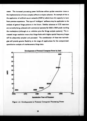
bit frame grabbers became available. T h is scale o f image re solution proved sufficient to analyse m any industrial problems and the com putational p o w e r produced an acceptable exe­ cution speed. A t this tim e , it became practical t o a tt e m p t fully autom a tic processing systems for a w ide variety o f fringe patterns.

N e w advances in V L S I (v e ry large scale in te g ra te d circuits) technology can be expected in the fu tu re as a consequence o f th e ra p id grow th th at has occurred in personal co m pu te r pow er. Figure 1.4 shows th e d e ve lo p m e n t of the microprocessors used in IB M and com patible P .C .'s in term s o f th e processor power in M IP S (M illions of Instructions Per S econ d ) against the in tro d u c tio n date of the chip . T h is graph shows an increasing rate o f grow th especially w ith t h e introduction o f th e i860

cessor. T h e increased processing power facilitates e ith e r quicker execution times or the implementation of more complex software analysis schemes. A n example of this is the application of artificial neural networks ( A N N ’s ) w h ic h have the capacity to learn from previous experience. T h is type o f 'intelligent' softw a re may be applicable to the analysis o f general fringe patterns in the future. S im ila r advances in C C D resolution are currently being achieved w ith commercial syste m s fo r 2048 x 2048 pixels reaching the marketplace (although at an inhibitive price fo r frin g e analysis system s). T h e in­ creased image resolution means th at fringe fields w ith higher spatial frequency fringes will be adequately sampled and processed. T h e co m bin a tio n of these tw o technolo­ gies w ill provide greater flexibility in the range o f applications for the computerised, quantitative analysis o f interferometric fringe data.

Figure 1.4: Developments in Personal C om p u ter Processing Power

1995

[image:29.363.35.321.13.410.2]

1.3 Automated Evaluation of General Fringe

Pat-terns

W it h th e availability o f co m pu te r hardware a n d high level program m ing languages, the theoretical ideas and algorithms for frin ge analysis could be im plem ented. T h is allows flexible system development and the incorporation o f new ideas in software. T h e com plexity o f th e analysis is then lim ited b y the algorithm used. Furtherm ore, th e autom ation of a fringe analysis system fr o m the operation o f peripheral devices to im age capture, data processing and sto ra ge m ay all be controlled by means of software.

T h e objective o f software analysis o f frin ge patterns is then to perform fully au­ to m a tic processing o f th e fringe data resulting in a contiguous phase distribution. A t this stage, it is w orth sum m arising the pro ble m s facing an autom a tic fringe analysis package. T h is list has been compiled w ith reference to work by Trolinger [31) and oth e r workers [32, 33).

A - i ) speckle noise, A - i i ) diffraction noise. A - i i i ) uneven fringe background, A - i v ) varying fringe contrast,

B - i ) unknown fringe sign,

C - i ) discontinuous and split fringes,

C - i i ) closely spaced fringes, C - i i i ) broad cloudlike fringes, C - i v ) extraneous fringes,

D —ii) lack o f a known reference position,

E - i ) the data reduction process should be fa s t and provide sufficient resolution of phase and the spatial detection o f th e phase.

The s e points m ay be grouped in to several categories. Item s A - l to A - 4 are caused by th e scattering characteristics o f th e surface under examination and any non-uniform ity in the interfering w ave fron ts. Th e s e problems are normally approached by pre-processing the fringe fields to a ttain b e tter and more uniform signal to noise ratio ( S N R ) over the entire field [32, 3 4 ].

T h e unknown fringe sign (ite m B - l ) m a y be reconciled by th e optical m ethod used (h eterodyne, quasi-heterodyne, carrier frin g e e tc .) [35], or by prior knowledge o f the experiment and hum an interaction (frin ge co u n tin g ). T h e latter is a non-autom atic process.

Items C - l to C - 4 specify the degree o f complexity o f th e phase data in the field. Problems m ay arise in the correct determ ination o f the interference phase for several reasons : when the phase changes rapidly and the fringe density approaches the N yquist sampling lim it o f the d e te cto r [33], or the fringes are very broad and some noise is present in th e data. O t h e r ambiguities m ay also be present such as discontinuous fringes. In this case different answers will be obtained depending on the route taken to relate th e phase at on e poin t to th at a t another [36, 37, 3 8, 39]. Extraneous fringes are due to extra co h e re n t waves being detected which add faint fringes to th e desired interference p attern.

T h e tw o points, D - l and D - 2 , are p a rtly caused by the experimental arrangement and the ‘view* o f th e object w hich is ob ta in e d . A point in the field which is known to have zero phase change, or equivalently n o m ovem ent, allows absolute measurements to be made. T h is is not always a necessary requirement, for example in N O T it is often the relative phase change across a specim en that is o f interest.

Finally, fast data processing and a specified resolution is required for the measure­ m ent m ethod to be industrially satisfactory.

of th e problems are solved by th e use o f the appropriate optical methods, e.g. the determination o f fringe order n u m b e rs. T h e extent to which the data quality is im proved and the phase determ ined is dependent on the com plexity of th e algorithm and th e initial quality o f th e d a ta . A fu rth e r consideration is the analysis speed which is especially relevant to th e industrial application o f the system.

1.3.1 Pre-Processing o f Fringe Data

T h e extent to which pre-processing m u st be applied is dependent on the optical m ethod used to generate th e d a ta . F o r fringe fields generated by classical specular interferom etry and some holographic fringe patterns th e data may be o f sufficient quality for direct phase calculation. However this cannot be guaranteed, and the case o f speckle interferom etry and m o ire systems need to be considered. Examples of interferometric, holographic, and E S P I fringe fields are given in figures 1.5 1.6 1.7. In each case the fringes are cosinusoidal and have been captured using a C C D camera and 512 x 512 x 8 bit fram e g ra b b e r. It is clear from th e form of these images th at th e noise content in each case is v e ry different. T h e noise may be assessed further by calculating the fast Fourier tra n s fo rm ( F F T ) of a row o f pixels in th e image. T h e resulting amplitude spectra are s how n in figure 1.8. T h e signal power in the high frequency range can be used as an estim ate of the noise co nte n t. T h e proportion of noise is seen to increase from interfe rom e tric to holographic to ES P I fringe images.

T h e methods of pre-processing frin ge data have been reviewed as part of a paper by Reid on a utom atic fringe analysis[32]. Further details on the m ethods are contained in references [33, 6 ]. It is assumed t h a t the fringe data has been digitised by a suitable cam era and fram e grabber.

T h e pre-processing technique t o be applied depends o n th e type o f noise present. W h e n the spatial frequency o f th e noise is higher than th a t o f the fringe data then a lo w pass filter m ay be applied. T h i s normally takes th e form of a window (o r kernel), w ith either the average o r median of the intensities contained within the w ind o w being determ ined. T h is va lu e is then used to supplant the intensity at the

R ow Spectra of Interferometric, Holographic and ESPI Data

Figure 1.8: A m p litu d e Spectra of Interferometric, Holographic, and E S P I Fringe

Data

[image:36.364.12.325.12.412.2]

centre of the w in d o w . T h e window shape is normally a square a rra y o f pixels or a cross. M ore sophisticated approaches have also been implem ented, f o r example the spin filter a lg o rith m s o f Y u [40]. T h is technique uses the average g r e y scale over a line in a specific d irection. T h e line is rotated, spun, around th e p o in t of interest until it lies as close as possible to a constant phase line. T h e ave ra ge value over the line is then assigned to the point in question. In this way, a more refined filtering of the data is p ro du ce d which reduces th e blurring effect of conventional square window filters. Square s h a p e d windows remain the most com m only used b e cau s e of the rapid execution tim es, approxim ately 30 tim es faster than the spin filter a lg o rith m .

A n effective re d u ction in speckle and electronic noise is produced b y all the m eth­ ods described. T h i s can be illustrated on the E S P I image in figure 1 .7 . B y applying fo ur successive ite ra tio n s of an averaging filter over a 3 x 3 w in d o w , th e image in figure 1.9 is p ro d u ce d . T h e spectra o f the same ro w in the original a n d the filtered images are shown in figure 1.10. T h e noise reduction achieved is a p p a re n t.

Similarly, in t h e case o f uneven illumination o r fringe co ntra st, th e fringe data m ay be separated fro m the background by a high pass filter. T h i s approach was implemented by B e c k e r [41] using regional averages. These values a re sm oothed over the w hole image a n d the result subtracted from th e interferom etric d a ta to form a m ore uniform b a ckg ro u n d intensity.

T h e alg orithm s above may also be implemented in frequency s p a ce rather than in th e spatial d om a in [42, 6 ]. T h is is achieved by evaluating the F F T o f a raster in the fringe data. A m a s k m ay be placed in th e fourier plane and then th e in ve rse transform taken to yield m o d ifie d intensity d a ta . B y appropriate choice o f t h e mask cut-off frequencies, th e desired noise reduction, high frequency or b a ckg rou n d variation, can be achieved on th e fringes [42].

O n e disad van tag e o f the frequency domain approach is the e x e cu tio n tim e which can be ~ 20 tim e s greater when com pared with the corresponding s p a tia l processing m ethod. T h is c a n be explained by com paring th e actual filtering processes being performed in each case. T h e F F T m e tho d produces the convolution o f the window function w ith th e im a ge , whereas the spatial domain approach on ly considers a small

Row Spectra of ESPI Data Before and A fter Filtering

region of the field ( 3 x 3 pixels) w ith unity am plitude for each p o in t in the window. T h e tim e p enalty in using frequency domain filtering has recently been overcome by using dedicated hardware [43].

T h e noise reduction algorithms as described above have a lim ite d usefulness when th e noise source has approximately th e same frequency as th e fringes. In this case it is very difficult to improve the data effectively. W h e n th e noise is stationary, i.e. not related to th e position o f the fringes, it is possible to s u b tra c t th e background variation by using tw o fringe images w ith a phase difference o f * radians between th em [31, 4 4 ]. T h e tw o images then represent th e same fringe field but a bright fringe in one im a ge becomes a dark fringe in the oth e r. B y p o in t-w is e subtraction of th e tw o fields, th e noise will be cancelled out. T h e process pro du ce s higher contrast fringes a t the expense of a more com plex optical arrangem ent.

In all the references cited in this section, the noise reduction algorithm has been suited to the d a ta concerned. Hence the analysis is a utom a tic o n ly if fringe patterns o f a sim ilar qu a lity are to be processed. A topic o f curre n t research is the automatic detection o f th e necessary degree o f smoothing.

1.3.2 Fringe Tracking

Some o f th e first codes to really tackle autom atic fringe processing were based on the idea o f ‘fringe tra ckin g'. T h e aim o f this technique is t o use an algorithm to a utom atically track the fringe maxima (o r m in im a ), see for exam p le [45, 4 6, 4 7, 48, 4 9, 3 2 ]. T h e fundamental concept is to examine a w indo w o f pixels around a given point. T h e average intensity is computed for all possible d ire ctio n s leaving the point in question, see figure 1.11. T o prevent the track from co ntinu a lly circling, only th ree of these directions from those possible are normally considered : th e original direction to reach th e point in question, and the directions either side o f t h e original direction [45]. If a fringe minima is to be traced, the m inim um o f the a verage intensities along these three directions is taken to reach a new point. T h e process is repeated until some criteria is satisfied or the edge of the image is m et.

3 * 3 Pixel Grid

Pixel to be Considered

Figure 1.11: Possible Direct

Previous Direction to Pixel in Question

ons to Track Fringes

3 Possible Directions to move

Forward

O th e r m ethods based on skeletonising the fringe data before fringe tra ckin g have been used [50, 51, 15]. Skeletonising normally results in a binary image achieved by the application of a threshold operator. T h e 'w h ite ' fringes in the image can then be thinned and tracked to form continuous lines representing frin ge maxim a. T h e analysis of a com bustion flame interferogram by Brya n sto n-C ross e t al [15] is interesting as a spatial resolution of at least 4000 x 4000 pixels w as required to adequately sample the fringe field. T h is w ork demonstrates th at fringe tra c k in g m ay be performed over a m u ch larger data space than the standard video resolution o f 512 x 512 pixels.

A n implementation of th e algorithm by B u tto n [4 5 ] has been made w ith a 5 x 5 pixel w indo w . T h e algorithm has been extended by considering the 16 directions shown in figure 1.12 and the a utom atic detection of a s ta rtin g point and initial direction for tra ckin g. T h e result for five fringes of the in te rfe rogram in figure 1.5 is shown in figure 1.13. A similar result can be obtained for th e holographic fringe data in figure 1.6, four tracked fringes are shown in figure 1 .14 . In this case the fringe data required filtering by a single pass of a 3 x 3 averaging w in d o w prior to fringe tracking. T h e sta rtin g points of th e tracked fringes were set a t j u s t below the sta rt o f the fringe data in th e image. T h e need for filtering can be dem onstrated by examining figure 1.15 w hich shows th e result when the same tra c k in g algorithm is executed on th e raw fringe data. T h is implies th a t a certain im age q u a lity is required for successful fringe tracking.

D u e to these problems, the development of fringe tra ck in g algorithms have fol­ lowed tw o separate paths : either the invention o f m ore sophisticated algorithm s for both im age enhancement and fringe tracking, or im p le m e ntin g semi- a utom a tic sys­ te m s requiring operator intervention. Both these approaches have been followed by different groups.

Yatagai et al [46] implemented a more critical te st fo r determ ining fringe maxima points by testing in several directions for each poin t. Based on the statistics o f speckle noise [2 0 , p.30 -3 6], it is more likely th at a dark speckle w ill occur in a bright fringe than a bright speckle in a dark fringe. Hence it is m ore d ifficult to track fringe maxima than m inim a in the presence of speckle noise and th e m ore sophisticated tests are

5 * 5 Pixel box for Determining Tracking Direction

Directions over which average of Pixel Grey Scales is Taken

Figure 1.12: 5 * 5 W indow for Im plem enting Fringe Tracking

necessary.

T h e problem of broken fringe tracks has been addressed by Liu et al [5 1 ]. In this work the ends o f fringe tracks which are not at the edge o f the image are identified. A sector is then defined using one such fringe end p o in t as the centre. If a second fringe end poin t is found within the sector then the tw o e n d points are joined.

In contrast Funnell [4 7 ], Yatagai et al [46] and P a rth ib a n [52] have developed interactive fringe tracking systems. T h e ir philosophy co nce d e s th at a fully a utom atic algorithm is not possible and consequently a hum an in te rfa ce is required to correct for mistakes.

Assum ing th at the fringe extrema can be tracked co rre ctly, there are still tw o disadvantages which are apparent for all fringe tra ckin g m e th o d s. Firstly, the fringe order num bers (p o in t B - l ) must be assigned m anually unless some prior knowledge can be utilised, o r carrier fringes have been added to th e o rig in a l fringe field. Secondly, phase data is only available on the fringe maxima and m in im a thereby restricting the use of the data especially for strain analysis w here spa tia l derivatives are required. T h is may be overcome by fitting a curve to the known frin g e maxima and/or minim a points, see for example [53, 54]. However this analysis is n o t usually employed due to the execution tim e required [32].

Fringe tra ckin g cannot therefore form a full solution t o th e autom atic analysis of interferograms, see section 1.3. However, the m e tho d is still used in classical lens testing interferometers because of the simplicity o f th e o p tic a l system required, and the high performance of fringe tracking algorithms on spe cu la r interferometric data (see figure 1 .1 3 ). A fringe tracking analysis system has so m e advantages in certain other cases.

i) W h e re an infrequent analysis is to be performed.

ii) T h e com plexity o f heterodyning optical systems is n o t practical. iii) In the analysis o f tim e average fringe fields (c o n ta in in g Bessel function

T h e first autom atic holographic heterodyne system was constru cte d by Dandliker and can produce data at a rate of approximately 1 second per point in the interferogram [28]. B y scanning the detector using a motorised x , y stage, a contiguous phase distribution can be obtained for the whole field at any required spatial resolution. T h e data collection and detector position are co m p u te r controlled. T h e lim it o f 1 second per point arises due to the re- positioning o f th e scanned detector and the tim e to log the detected phase data. It may be possible to increase the data collection rate by continuously scanning a detector across th e fringe field and reading the phase data a t intervals providing th at the stability o f th e optical system can be m aintained. A different approach was adopted by Massie [5 5 ] w here an image dissector camera was used to select w hich part of the interference field is sampled at any poin t in tim e. T h e system constructed allowed data collection at 5/j s per point. The refore , to cover th e n u m be r o f points available in a 512 x 512 fram estore, i.e. 262144, requires approximately 1.3 seconds.

T h e advantages of heterodyne phase m easurem ent are th e very small phase differ­ ences w hich may be resolved unambiguously. U p to o f a fringe can be achieved. T h e spatial resolution is high and only lim ited by the motorised traverse stage (o r image dissector ca m e ra ) and the characteristic speckle size in the image. Som e noise im m un ity is also gained as the phase to be m easured is independent of extraneous fringes (ite m C - 4 ) w hich are not modulated a t th e beat frequency, and the interfering wavefront amplitudes (item s A - 3 and A - 4, see equation 1 .6 ).

Despite these benefits, heterodyne systems are confined to a stabilised laboratory bench [56]. T h is is due to the stability requirem ents o f th e reconstruction optics over the duration o f the data read-out and the need for a ccu ra te hologram repositioning after development. C learly this is not appropriate for perfo rm in g rapid measurements in an industrial environm ent. Th e re is no facility to pre-process the fringe data (p o in ts A - l to A - 4 ) and hence successful analysis is dependent o n achieving sufficient signal in th e detected intensity at the recording stage o f the interferogram [57].

1.3.3 Autom ation o f H eterodyne Phase Analysis

T h e autom ation of quasi-heterodyne analysis systems was a p p a re n t after the work by B ru n in g et al. In general a com puter system is linked to : a C C D video camera via an image frame grabber, and a device fo r varying the phase of the fringe field. Synchronisation o f the image capture system an d fringe field phase is achieved through software. It has been shown by subsequent w orkers th at th e set o f phase stepped images (typically three, four, or five, see section 1 .1 .2 ) can be ca p tu re d in consecutive video frames (see for example [8 ]). T h is is d on e by moving th e phase shifting device in the read-out tim e of the C C D camera. H e n ce digital image ca p tu re requires ^ of a second, where n is the number of images.

O n ce the data is in digital form, the data processing m ay be achieved by a sequence of software functions. T h is allows flexibility in th e analysis a n d independent fringe pre-processing (section 1 .3 .1 ) followed by phase co m putatio n. M a n y phase calculation algorithms are available and have been reviewed by Creath a n d W yk e s [58, 56]. As described in section 1.1.2, the resultant phase is evaluated m o d u lo 2 x . T h e image formed is called a 'w rapped' phase map. T h e w ra p pe d phase m a p corresponding to figure 1.6 is shown in figure 1.16 where the phase values b etw een —* and x have been encoded as grey scales from 0, black, t o 2 5 5, white. T h e cosinusoidal images were smoothed using a 3 x 3 averaging filter prior to calculation o f the wrapped phase values.

T h e a utom atic processing of a wrapped phase m ap, i.e. ‘ phase unwrapping’, will be discussed after the following section.

T h e advantages of quasi-heterodyne analysis are :

i) th e rapid, a utom atic data acquisition w h ich directly yields th e fringe data in a digital form,

ii) and the facility for software analysis.

T h e phase measurement resolution is also high, up to o f a frin ge [58], whilst the spatial resolution is fixed by : the num ber o f pixels in the d ig ita l frame grabber (o r

1.3.4 Automatic Quasi-Heterodyne Fringe Analysis