Bayesian applications in econometrics

BAYESIAN APPLICATIONS

IN ECONOMETRICS

A thesis presented for the degree of

Doctor of Philosophy

in Economics

at

the University of Canterbury

Christchurch, New Zealand

by

D.E.A. Giles

"

\3CJ

'GI;-l'l.

\915

CHAPTER

1.

II.

ABSTRACT

INTRODUCTION

CONTENTS

PAGE

1 3

I. Introductory comments. 3

II.

BASIC

1.

II.

III.

IV.

V.

(1) General background . . . . . 3

(2) Bayesian methods in econometrics 6

Outline of the thesis • • . 9

RESULTS 0

· ·

.

12

Definitions

_·

. . . . . 12

Bayes' theorem . . . 13

Estimation

_·

_{· ·}

_{• • • 1 5}

Prediction

_{· · ·}

.

· . . . 17

Model comparisons • • 0 18

III. A M.S.E. COMPARISON OF TWO M.E.L. ESTIMATORS

FOR THE MULTIPLE REGRESSION MODEL ₂₁

21

23

10 Introduction

II. Preliminary results.

A

III. Comparing

a

and

a ..

IV. Further analytic results

(1) Speci cation of

13

• • • • • • • 26

32

33 (2) Speci fica tion of A . . . 37

(3) Multicollinearity and precision. . 48

V. A special prior p.d.f.

VI. A test statistic

(1) A formal test

(2) An ad hoc test

VII. Conclusions.

· . . . Sl · . . . 53 53 59

CHAPTER PAGE

IV. B'AYESIAN SEASONAL ADJUSTMENT OF ECONOMI C

TIME SERIES . . . .

I. Introduction.

81 81 82

II. Explaining seasonality

III. Statistical properties _{· . . ". . . 83}

IV. The systematic component. 85

V. Estimating the seasonal influence 87

VI. Model comparisons

VII. Regression relationships with seasonal

data . . . .

VIII. Conclusions

V. BAYESIAN ANALYSIS OF DISTRIBUTED LAG MODELS:

A SURVEY

I. Introduction

II. Infinite lag models

(1) Rational lags

(2) Other contributions

III. Finite lag models

IV. Conclusions

VI. DISCRIMINATING BETWEEN AUTOREGRESSIVE FORMS:

A MONTE CARLO COMPARISON OF BAYESIAN AND

AD HOC METHODS

.

. .

I. Introduction

II. B.P.O. Analysis

_{· ·}

I I I . The Monte Carlo study

_·

.

_·

(1) M1 is true

.

. . · .

(2) M_Z is true

_{· . .}

(3) Limitations of the tests

.

90

92

94

95 95 97 97

100

101

104

106

106

111

114

115

117

IV. The choice of data and parameters

_{· ·}

119

( 1) Exogenous variable

_·

_{· ·}

119

(2) Parameter values 119

( 3) Random disturbances

_·

120

(4) Initial value of y

_·

_·

_{· · ·}

_{· ·}

121

V. Results

. .

.

. . · · ·

_{· ·}

_·

_·

_·

121

(1) Ml is true

_{· · ·}

_{· ·}

_{· ·}

_·

_·

122 (2) M2 is true

.

_{· ·}

_·

_·

_{· · · ·}

128

( 3) Summary

_{· · ·}

_{· '.}

_·

_·

133

VI. Conclusions

.

_·

_·

_·

_·

_·

_·

135

VII. BAYESIAN INFERENCE AND THE RESTRICTED

ALMON ESTIMATOR. PART I: THEORETICAL RESULTS 137

I. Introduction 137

II. The classical P.A.E. _{· . 138}

(1) Estimation _{· 138}

(2) Linear restrictions . _{· . 139}

(3) A Critique _{· . . 140}

II I. Bayesian considerations . .

IV. Re-parameterizing the model

· . 143

· 147

V.

VI.

VII.

Bayesian estimation . · . 151

(1) Serially independent errors . . . 151

(2) Serially correlated errors 156

Random L

.

.

.

.

..

. .

.

. .

. .

_{· . 159}

(1) Serially independent errors . . . 160

(2) Serially correlated errors 163

Model comparisons . . . · . . . 165

(1) Computation of th.e B.P.O.. . 165

(2) A Qualification . . . . . 169

CHAPTER PAGE

VIII. BAYESIAN INFERENCE AND THE RESTRICTED

ALMON ESTIMATOR. PART II: AN APPLICATION TO

CURRENT PAYMENTS FOR NEW ZEALAND IMPORTS 172

I. Introduction . .

II. Data . .

I II. Seasonal adjustment

IV. Estimation . . . .

V. Prior knowledge

(1) The model space

(2) The parameter space

VI. Posterior distributions

(1) L fixed and known; independent

.

.

.

(2) L fixed and known; correlated

. . . .

errors

. .

.

errors

. . .

(3) L random; errors serially independent

(4) L random; errors serially

correlated .

· . '.

serially

·

·

·

.

.

serially

· · · . .

172 173 175 177 l7~ 180 180 183 184 185

· . . . 187

VII. B.P.O. and point predictions .

189

191

191 (1) B.P.O. analysis

(2) Point predictions

· . .'

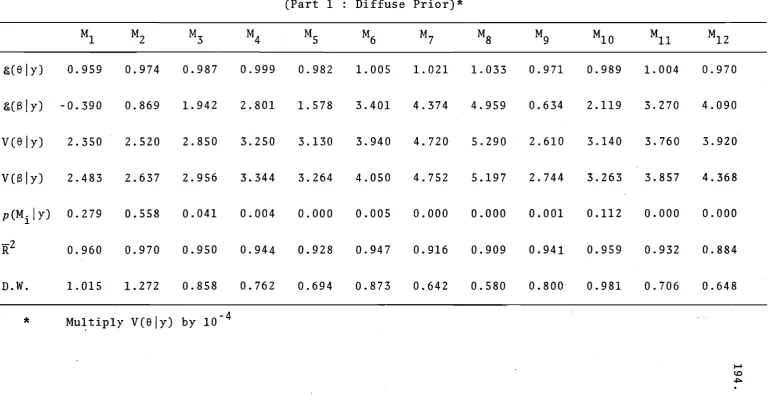
192

VI I I. Resul ts 193

IX.

(1) Discussion of tabulated results 193

(2) Diagrammatic resul ts . . . 221

(3) Appraisal of the Bayes-Almon

estimator

(4) Economic implications

Concluding remark

232

236

IX. SUMMARY AND CONCLUSIONS . ACKNOWLEDGEMENTS

. .

REFERENCES APPENDIX

. . .

. .

. . . .

.

.. I: SOME USEFU L RESULTS .

APPENDIX II: SOME RESULTS WITH THE ONE~

REGRESSOR MODEL . . . . . APPENDIX III: LAG DISTRIBUTION SHAPES. APPENDIX

APPENDIX

IV: RAW DATA FOR CHAPTER VIII

V: SEASONALLY ADJUSTED DATA

238

242 244 253

TABLE II I. VI.1 III. VI. 2

III.VI.3 III. VI. 4

I II. VI. 5

I II. VI. 6

III. VI. 7

I II. VI. 8

I I I. VI. 9

III.V1.10 III. VI. 11 III.VI.12

III.VI.13 I II. VI. 14 . VI. IV.1

VI. V. 1

VI. V. 2 VI. V. 3

VI.V.4

VI. V. 5 VI. V. 6 VI. V • 7

VI. V. 8

LIST OF TABLES

2 .

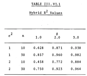
Hybrid R values

. . .

.

PAGE

· . • 68 71

· . . 71

72

a

=

1.0; 0 2

=

1.0; n

=

10

a

=

1.0; 0 2

=

1.0; n

=

30

a

= 2.0; 0 2

=

1.0; n

=

10

a

=

2.0; 02

=

1.0; n

=

30

a

=

3.0; 0 2

=

1.0; n

=

10

a

=

3.0; 0 2

=

1.0; n

=

30

a

=

1.0; 02

=

2.0; n

=

10

a

=

1.0; 0 2

=

2.0; n

=

30

a

=

2.0; 0 2

=

2.0; n

=

10

a

=

2.0; 0 2

=

2.0; n

=

30

B

=

3.0; 02

=

2.0; n

=

10

a

=

3.0; 02

=

2.0; n

=

30

Estimated power functions Hybrid R2 values . . . .

72

• • • 73

• • • 73

• • • • 74

• • • 74

• • • • • 75 75

• • • 76

. • • • 7 Q

77

121 M1 true; y = 0.90; p = 0.30 . . . 124 M1 true; Y

=

0.90; p

=

0.60

Ml true; Y

=

0.90; p - 0.90

G < 5%

.

. .

.

.

..

. . .

.

.

. . .

. .

MZ true; B = 0.09; A

=

0.90

M2 true; B

=

0.45; A = 0.50

M2 true;

a

=

0.81; A

=

0.10 . . . .

~[PTfT + p (I 1) ]

125

126

127

130

VIII.VIII.1 Part 1: diffuse prior.

VIII.VIII.2 Part 1: diffuse prior . .

VIII.VIII.3 Part 1: diffuse prior

. . .

.' 131 132 134 194 195 196 197

VIII.VIII.S Part 1 : loose prior

_{· ·}

_{· · · ·}

198 VIII.VIII.6 Part 1 : loose prior

_{· · ·}

_·

_{· ·}

₁₉₉

VIII.VIII.7 Part 1: tight prior

_·

_{· ·}

_·

₂₀₀

VIII.VIII.8 Part 1 :: tight prior

_·

_{· · ·}

₂₀₁

VIII.VIII.9 Part 1 : tight prior

_·

_{· ·}

_·

₂₀₂

VIII.VIII.10 Part 2 : diffuse prior

_·

_·

_{· ·}

₂₀₃

VIII.VIII.11 Part 2 : diffuse prior

_·

₂₀₄

VIII. VIII.12 Part 2 : diffuse prior

_·

_·

_·

_20S

VIII.VIII.13 Part 2 : loose prior

_{· · ..}

_·

_{· · · · ·}

₂₀₆

VlIl.VIII.14 Part 2 : loose prior

_{· ·}

_·

_{· · · ·}

207

\

VIII.VIII.IS Part 2 : loose prior

_·

208

VIIl.VlII.16 Part 2 : tight prior

_{· · ·}

_·

209

VIII.VIII.17 Part 2 : tight prior ₂₁₀

VIII.VIII.18 Part 2 : tight prior 211

VIIl.VIIl.19 Part 3

_{· ·}

_·

_·

_{· ·}

_·

212

VIII.VIIl.20 Part 3:

_{· ·}

_{· .}

_{· ·}

_·

_{· · ·}

_·

213

VIII.VIII.21 Part 3

_·

_·

_·

_{· · · ·}

214

VIII.VIII.22 Part 4

_{· · ·}

_·

_{· ·}

_·

21S

VIII.VIII.23 Part 4

_{· · · . · · ·}

_·

_·

_·

216

LIST OF FIGURES

FIGURE PAGE

I I 1. IV.l Effects of varying

a

_·

_{· ·}

_·

_·

_·

_·

34

I II. IV. 2 A as a function of

_a

_·

_{· · · ·}

_·

_·

36 I I I. IV. 3 An extreme curve decolletage

_·

_·

_{· ·}

_{• 42} I II. IV. 4 Effects of varying cp when

s*' (X'X)S*

> 0 2

· · · ·

_·

· · ·

_{· 44}

III.IV.S Effects of varying cp when

S*' (X'X)S*

=

0 2

·

,.

·

·

·

_{· ·}

·

_{• 44}

I II. IV. 6 Effects of varying cp when

S*' (X' X) S*

< 0 2

.

. ·

·

·

·

_{· ·}

_{• 44}

II I. IV. 7 A as a function of cp

·

·

· ·

· ·

· 47 III.V.l The curve decolletage when A a:

(X'X)

_{· S 3}

I I 1. Vr.l Estimated power curves

_{· ·}

78

VIII.VIII.l _{Part 1, M2 (diffuse prior)}

_·

_{· ·}

222 VIII.VIII.2 _{Part 1, M2 (loose prior)}

_·

_·

_{· ·}

_{· 222} VIII.VIII.3 _{Part 1, M2 (tight prior)}

_·

_{· ·}

_{· · ·}

_{· 222} VIII. VIII. 4 _{Part 1, M2 (posteriors)}

_{· ·}

· 223 VIII.VIII.S _{Part 1, M2 (joint} po~teriors)

_·

_·

_·

_{· 223}

VIII.VIII.6 _{Part 2, M3 (diffuse prior)}

_·

_{· 224}

VIII.VIII.7 Part 2, _{M3 (loose prior)}

_·

_{· ·}

_{· ·}

_{· ·}

224 VIII.VIII.8 _{Part 2, M3 (tight prior)}

_·

_{· ·}

_{· ·}

_·

_·

225 VIII.VIII.9 Part 2, _{M3 (comparative posteriors). · 225}

·VIII.VIII.I0 Part 3, SI (diffuse prior)

_{· · ·}

_{· ·}

· 226 VIII.VIII.l1 Part 3, SI (loose prior)

_·

_{· · ·}

· 226 VIII.VIII.12 Part 3, SI (tight prior)

_{· · · ·}

_·

227

VIII.VIII.13 Part 3, SI (comparative posteriors). · 227

VIII.VIII.17

A.1

A.2 A.3 A.4 A.S A.6

Part 4, Sl (posteriors) . . . .

P

=

1

P > 2

P _-> 2

P _-, > 2

P > 3 P > 3

_·

-231

260 260

261

261

261 261

P > 3

_·

A.7 261

P > 4

_·

A.8 _- . 261

A.9 Seasonally adjusted current payments. 267

[image:10.539.44.477.72.789.2]

1.

ABSTRACT

The thesis considers several related aspects of

Bayesian inference in econometrics. Particular attention

is given to model-comparisons, distributed lags, and the

sampling properties of estimators.

In Chapter III the natural-conjugate Bayes (8) and "

Ordinary Least Squares (8) estimators for the linear model

are compared, and a condition is derived and investigated

under which 8 is preferred to 8 in terms of matrix mean

squared error. In a limiting case a test statistic is

obtained and shown to be related to another well-known test.

Two observable substitute statistics are shown to be

consistent but upward-biased. The bias is studied in a

limited Monte Carlo experiment.

Bayesian inferential methods are advocated in

Chapter IV for the seasonal adjustment of economic

time-series. This is motivated by Chapter III and the application

in Chapter VIII. A well-known classical procedure is shown

to be a special case of the Bayesian method.

Bayesian analyses of distributed lag models are

surveyed in Chapter V, and Chapter VI considers the problem

of discriminating between a Koyck distributed lag model

and a regression model with autocorrelated disturbances.

A Monte Carlo study compares several interpretations of an

ad hoc rule-of-thumb proposed by Griliches with Bayesian

Posterior Odds analysis, and the latter is found to be

Chapters VII and VIII present a Bayesian

inter-pretation of the Almon estimator, treating theoretical

results and an application to some New Zealand data.

The theory generalizes that of Zellner and Williams,

special attention being paid to: prior information;

unknown lags; model comparisons; and autocorrelation.

Although the methodological problems associated with the

classical Almon estimator are overcome, the computational

cost is increased substantially.

The evidence presented suggests that several

econometric problems may be handled more satisfactorily

3 .

CHAPTER I

INTRODUCTION

I. INTRODUCTORY COMMENTS

(1) General Background

In recent years the theory of mathematical statistics

has been liberated to some extent from the firm grip of the

"frequentist" (or "classical") school associated with

Sir Ronald Fisher in the United Kingdom, and with J. Neyman

and E.S. Pearson in the United States. 1 There has been

renewed interest in an old principle first suggested by

Thomas Bayes in 1763.

Although Bayes is well known for the theorem which

bears his name, in fact it seems that he has even closer

links with the modern "Bayesian" school, in that he shared their concept of probability.2 Modern Bayesians differ

from the frequentists by adopting a subjectivistic

(personalistic) view of probability, rather than defining

a probability as a long-run frequency. Although the use of

Bayes' Theorem is important in modern Bayesian analysis, it

is also used (correctly) in various contexts by frequentists.

The Bayesian approach draws on the contributions of

de Finetti (1937), (1972); Ramsey (1950); Savage (1954),

(1961); and Jeffreys (1961). This subjectivistic

inter-pretation makes it meaningful to attach probabilities to once-and-for all events, parameters, hypotheses or models.

1. See Bartlett (1965); Plackett (1966); Lindley (1965).

The value of a subjective probability represents a personal

degree of belief, based on the individual's present state of

knowledge. As data are observed, this state of knowledge

changes, and the a priori degrees of belief must be updated

to the a ppsteriori state. This updating is effected

through Bayes' Theorem, thus introducing the basic principle

of "learning from experience". The process may continue

sequentially if additional data become available. The

previous a posterior state then becomes the new a priori

state, and Bayes' Theorem is applied again, etc ..

Expressing this somewhat differently, a priori

information is combined with sample information, the total

amount being summarized in the resulting a posteriori

distribution. This distribution contains all of the

available information. However, Bayesians often wish to

make decisions on the basis of the posterior distribution3 ,

and at this stage the loss structure of actions is taken

into account explicitly. Being based on the earlier work

of von Neumann and Morgenstern (1947) and Wa1d (1950),

Bayesian decision theory pursues the principle of acting

to maximize expected utility.

The Bayesian philosophy should be (and has been)

scrutinized on at least two fundamental levels. First,

the concept of subjective probability itself4 has' prompted

a heated debate. An individual's (subjective) probability

of the outcome of an event is determined by the least

odds at which he is prepared to bet on that outcome, such

3. For example, one may wish to draw statistical inferences, such as choosing a point estimate.

5.

bets being measured in terms of utility. In all but the

simplest of situations the introspection required to

determine the prior distribution precisely would be

enourmous. 5

Secondly, there is the explicit introduction of a

model of "learning from experience", arising with the use

of Bayes' Theorem. This view of the learning process is

in direct conflict with that advocated by Popper (1965),

Kuhn (1962) and Feyerabend (1965), for example. In their

view, we learn from our mistakes, and progress as a result

of criticism and by trying to refute earlier propositions. 6

The philosophical debate surrounding Bayes' Theorem

is as old as the theorem itself, and the controversy over

the subjective view of probability is by no means resolved

either. These issues are of fundamental importance and

will undoubtedly continue to pose problems for philosophers

of mathematics for some time.

However, such matters are not the subject of this

thesis, and are raised here only to provide a setting for

what is to follow. Despite the controversy which still

surrounds the Bayesian school of statistical thought, its

adherents have made many important contributions in recent

years, and its acceptance appears to be spreading. 7 _Thus,

5. See P1ackett, op.cit., pp.252-253; Raiffa and Schlaifer

(1961), pp. 59- 62 .

6. For example, see Rothenberg (1969), pp.200-204.

7. To some extent this is reflected in the appearance of texts on mathematical statistics which are written

primarily from a Bayesian viewpoint. For example,

for the purposes of this thesis we accept the

meaningful-ness and usefulmeaningful-ness of the Bayesian philosophy, at least

in certain situations, and consider some aspects of its

use in econometric theory.

(2) Bayesian Methods in Econometrics

The recent developments in mathematical statistics

have been reflected in several of the disciplines based on

this theory, one of these being econometrics. By virtue.

of its historical development, econometrics is firmly

based on the principles of frequentist theory, though

lately there has been increasing interest in the use of

Bayesian methods for analysing econometric problems.

The supporters of a Bayesian approach in econometrics,

notably Arnold Zellner, have argued convincingly for its

wider adoption. a If there is one principal self-supporting argument advanced by these Bayesians it is that their

approach is based on a simple and unified set of principles

which provides the means for inference and decision-making

in a wide variety of situations. According to its adherents,

it is in this respect that the Bayesian approach in

econometrics stands above its non-Bayesian rivals, the

latter being seen as a collection of "ad hockeries".

The specific advantages of the Bayesian approach to

econometric analysis are essentially those that apply at

a more general level in mathematical statistics. These

advantages have been summarized well by Zellner (1969), and

8. For example, see Zellner (1969). Much of Zellner's

7 .

relate to the main areas of econometric theory: estimation;

hypothesis testing; prediction; control; the incorporation

of prior information; the handling of "nuisance" parameters;

and specification analysis.

Of prime concern in econometrics9 _{are the two. major}

areas of inference: estimation, and hypothesis testing.

In the former, the main contribution of the Bayesian

approach is that unknown parameters are treated as random

variables and are assigned prior probability density

functions (p.d.f. IS) or probability mass functions (p.m.f. IS).

Sample information is introduced via the likelihood function,

and then posterior p.d.f. 's (or p.m.f.'s) are produced by

means of Bayes' Theorem. Once the loss structure is made

specific, the posterior distributions form the basis for

point or interval estimation1o , if such estimates are desired. For example, see Tiao and Zellner (1964).

With regard to the latter, the subjectivistic

interpretation of probability makes it meaningful to

compare non-nested models or hypotheses. In general, such

comparisons cannot be formalized within the frequentist

framework, though unfortunately ad hoc attempts are often

made. Major contributions to the Bayesian theory of

model comparisons have been made by Thornber (1966),

Geisel (1970), Lempers (1971), and Gaver (1974). Bayesian

and non-Bayesian methods in this area have been surveyed

9. Again, the comments here in general apply to math-ematical statistics, not just to econometrics.

10. In contrast, classical theory treats the parameters

by Gaver and Geisel (1974). Again, the analysis relates

to any parametric statistical models, but the presentation

by these authors centres on economic problems, and

economlc applications are given.

There are many troublesome areas of traditional

econometric theory which may be handled formally and

efficiently by Bayesian methods. Examples are the problems

of model comparisons; the handling of "nuisance" paramet·ersl l;

specification analysis12; and distributed lag models 13 , to

name a few. As might be expected, however, these gains are

not without cost.

For example, although it is helpful to have a

formal means of using prior knowledge, it may be very

difficult to formulate a satisfactory prior p.d.f.

(or p.m.f.) in practice. In such cases a Bayesian might

suggest trying a variety of prior distributions (including

one devoid of informational content 14

) in order to test

the sensitivity of inferences to the choice of prior p.d.f ..

Further, in practice Bayesian methods in econometrics

(and elsewhere) may have to be limited to rather simple15

models, unless the prior p.d.f. can be chosen in such a way

that it can be combined with the likelihood function

11.

12. 13. 14.

15.

See Zellner (1971), pp.21-22. See Lempers, op.cit., pp.47-65. See Chapter V of this thesis.

For a discussion of prior ignorance, see Zellner

(1971), pp.41-53, or Box and Tiao, op.cit., pp.25~60.

9.

analytically. 16 In general, numerical approximations must

be used when integrating to normalize the posterior p.d.f.

and to obtain its moments. In such cases the computa.:.

tional cost of even simple techniques as Simpson's rule

is prohibitive in parameter spaces of even moderate dimens ion. 17

However, as already noted, a wide range of

important econometric problems which cause difficulties·

in a frequentist setting, are well suited to Bayesian

analysis. Despite conceptual and practical difficulties,

the Bayesian framework has much to offer when analysing

problems of this type, and considerable progress has been

made in a variety of areas.

A belief in this (limited) usefulness of Bayesian

inference in econometrics underlies this thesis.

II. OUTLINE OF THE THESIS

The thesis considers a number of related problems

concerned with the use of Bayesian methods of inference

in econometrics. The layout is as follows. Chapter II

contains some basic notation and results related to

Bayesian estimation, hypothesis testing ,and prediction.

16.

17.

Two such types of prior p.d.f. are Jeffreys'

"diffuse" prior, and the Natural-Conjugate priors suggested by Raiffa and Sch1aifer, op.cit., pp.43-76. Very roughly, the processing time w~en applying

This material is drawn primarily from Zellner (1971;

Ch. 2, 3), and from Geisel (1970; Ch. 1, 2), and is. used

repeatedly throughout the thesis.

The rest of the thesis falls broadly into two

sections. Chapter III is quasi-Bayesian in philosophy,

lying between the frequentist and Bayesian school~, in

that it considers the sampling properties of certain Bayes

estimators. Using general I8 _{Mean Squared Error (M.S.E.) ·as}

a basis, two estimators for the linear regression

model are compared in various situations. This M.S.E.

basis forms part of the motivation in Chapter IV for a

Bayesian interpretation of the problem of seasonally

adjusting an economic time-series. The approach used here

amounts to a particular application of the usual Bayesian

methods of inference in parametric models.

The second, and major section of the thesis centres

on the Bayesian analysis of distributed lag models. Such

models have been analysed already by different Bayesian

methods under various conditions, the relevant literature

being surveyed in Chapter V. One of the main reasons for

concentrating on this type of model here is that it raises

a wide variety of econometric problems which are very

difficult to solve by classical methods, but which may

be handled more successfully by adopting a Bayesian approach.

Chapter VI analyses a particular problem of model

discrimination which arises with certain infinite distr~buted

lag models, and compares Bayesian Posterior Odds (B.P.O.)

11.

analysis with an ad hoc approach.

The Polynomial Approximation (Almon) estimator

for finite distributed lag models has received a lot of

attention in the literature since its conception, partly

as a result of the methodological problems which it poses

for frequentists. A general Bayesian interpretation of

this estimator is developed in Chapter VII, this being

an extension of the earlier contribution by Zellner and

Williams (1973). This estimator is applied to some New

Zealand data in Chapter VIII. Some concluding remarks

CHAPTER II

BASIC RESULTS

Here, and throughout the thesis the symbol p

denotes any general prior or posterior p.d.f. or p.m.f.,

regardless of mathematical form. It may relate to

parameters, observations, or models, but the meaning will

be clear from the context in which it is used. l

I. DEFINITIONS

We define four spaces required for a discussion of

Bayesian decision theory:

The sample space, Y

=

{y}, is the set of all possible

values of the sample observations for the experiment of

interest.

The _~---~~-, A

=

{a}, is the set of possible actions

related to a particular decision problem.

The model space,

Wl.

=

{M}, is the set of poss ib Ie mode Is or

hypotheses for the experiment being considered. 2

The parameter space,

n

i

=

rei}' for the ith. model in

11t

is the set of unknown parameters associated with that model.

Both ~ and the ni's are stat~ spaces in the .usual

terminology. Further, a parametric statisti~al model of a

1.

2.

Detailed descriptions of the basic Bayesian framework are given by Raiffa and Schlaifer, op.cit., de Groot, op.cit" and Box and Tiao, 0E.cit ..

This space is restr1cted to be finite or countable, for

asons described below. However, this restriction can

13.

stochastic process is a family of data densities,

depend-ent on a (usually finite) number of parameters and a

specified set of predetermined variables, and a prior

density for the parameters of the data densities.

For each model in

nt,

the data density is given by

p(yla.

,M.), which when viewed as a function of the unknown

1 1

parameters is the likelihood function, Q (a. ly,M.). The

1 1

prior p.d.f. (or p.m.f.) for the parameters of Mi is giv~n

by p(a·IM.). Finally, a prior p.m.£' is defined over the

1 1

elements of

m,

so that the prior mass of the ith. model is

p (M.) . 1

II. BAYES' THEOREM

The conditional (on the model) data density is

obtained as

P(yIM.)-= f p(yla.,M.)p(e·IM.)da.,

1 ~. 1 1 1 1 1

1

and the marginal data density is

p(y)

= Ep (y 1M. ) p (M. ) . 1 1

1

ILI!.l

ILII.2

The~ applying Bayes'Theorem, the (joint) posterior

p.d.f. for the parameters of the ith. model is

p(a·ly,M.) = {p(e·IM·)p(yla.,M·)}/p(yIM.)

1 1 1 1 I I I IT.IL.3

p(6.ly,M.) iXp(a·IM.)2(9·ly,M.)

1 1 1 1 1 1

where the proportionality constant is 3

I

-1

{f PCa.IM.)2(6. y,M.)d8.}

Q. 1 1 1 1 1

1

Further, the posterior probability of the ith.

model is given by

or,

p(M.ly) iX p(M.)p(yIM.)

1 1 1

I1.I1.4

where the proportionality constant is

{~p(M.)p(YIM.)}-l.

. 1 1

1

In many instances, attention centres on one (or a

subset) of ~he parameters in the vector ai' In such cases,

- - - " " - - - posterior p.d.f. 's for these parameters may be

derived.

a. '

₁

Q.

1

Then,

Partition a. and Q. such that

1 1

3, Here and throughout the thesis the notation is simplified by using the single symbol f even for

multi-dimensional integrals.

15.

where eli E Q1i; and a symmetric result holds if p(ezily) is required. Such integration is also useful for

eliminating "nuisance" parameters, once their influence

on the posterior p.d.f. for the remaining parameters has

been accounted for.

III. ESTIMATION

We define a decision rule, d, as a function mapping

Y to A. Further, a loss function Lis a real function

describing the loss of utility (in the von

Neumann-Morgenstern sense) resulting when action a is taken for a

particular true state of nature. This state of nature

will be a point in Q. here, but in Section V below it 1

will be a model in

nt.

Thus, here L maps (Q. x A) to

1

[0,00). The notation L(8.,e.) denotes the loss incurred

1 1

when e_i is the true state of nature, and e

i is the point estimate lf _{of e ..}

1

The minimum expected loss

(ME1J

rules is to choose

e. such that 1

A

f L(8. ,8.)p(e·ly,M.)de.

Q. 1 1 1 1 1

1

is minimized. If this integral is finite, then the Fubini

Theorem may be applied, and it can be shown that 8_i is a

MA~ estimate iff it is a Bayes estimate of e .. As such, 1

4. _{The selection of 8 i amounts to taking some action, a.}

9. minimizes average risk. However, in some cases the

1

M.E.L. estimate exists when the Bayes estimate does not,

and so in this thesis we concentrate on M.E.L. decision

rUles. 6 _{As it is well known}7

, if L is positive definite quadratic then the M.E.L. estimate, 6., is the mean of the

1

conditional posterior p.d.f. for a_i :

A

6i

=

_{&(aily, Mi )·}

Now, let ~' _r denote the rth moment about zero for

6· . ₁ So,

~'

=

r

e~p(a·ly)da.

r Q. 1 1 1

1

=

~.

e

I

U:p (e i

I

y, M i) p eM i

I

y) ] d a i

1

= I:p(M·ly)

r

a:pca·ly, M.)da.

. 1 ~ 1 1 1 1

1 ~6'

1

say. II. 111.1

Thus, under the above loss function the marginal M.E.L.

estimate of

e.

is

1

=

I:p (M.

I

y) &(

e .

I

y, M.)

. 1 1 1 11.111.2

1

Let ~r _{denote the rth moment about the mean for a i . Then}

it is well known that

11.11I.3

6. Here we are following Thornber, op.cit.; Geisel,

~it.; and Gaver, op.cit.. .

17.

Combining 11.111.1 and 11.111.3,

11.111.4

Thus,

v(eily)

=

~P(MiIY)[V(eily,Mi)+(&(aily,Mi))2]

1

-

[~P(Mily)&(aily,Mi)]2

1

11.111.5

IV. PREDICTION

Let YFEYF be a vector of as yet unobserved (future)

observations for the endogenous variable of the stochastic

process. Then the predictive p.d.f~ for YF is

p(yFly)

=

~p(YFly, Mi)P(Mily),

1

II.IV.1

where P(Mily) is obtained in 11.11.4,

p(yFly,M.)

=

J p(yFIS. ,M. ,y)p(e·ly,M.)de.

1 Q. 1 1 1 1 1

1

I I. IV. 2

In this case, the loss function maps (YF x A) to

~ A

[0,00), and L(YF' YF) denotes the loss incurred when YF is chosen as the point estimate of the unknown YF' Again,

"

"-J L(YP,yp)p(Yply,Mi)dyp

Yp

is minimized8 _{, and results analogous to 11.111.2 and II.III.S} apply here.

V. MODEL COMPARISONS

Let M. denote the action of selecting the jth.

J

model from 1Y/,. In this case L maps (m x A) to [0,(0).

Since M is assumed to be countable, the MEL. and Bayes

rules are equivalent9 _{, and M. is chosen from~ iff}

1

EL(M ,M.)p(M Iy) < EL(M ,M.)P(M Iy)

r r 1 r r r J r

for all j~i.

II.V.I

If attention focuses on just two of the models in

~, then the B.P.O. relating Mk and M_j are

{P(MiIY)/P(Mj Iy)}

=

{P(Mk)/PCMj)}{p(yIMk)/P(yIM_{j )},}

II.V.2

which depends on the prior odds and the ratio of weighted

likelihood functions, the latter being obtained from

11.11.1. The B.P.O. are independent of

pey),

so there is

no need to specify the full extent of

m

if only Mk and M_j

are of interest. Although the B.P.O. are unaffected by

the presence or absence of other models as long as the

prior odds are unaffected, clearly any individual posterior

8. See Zellner (1971), p.30.

19.

probability depends on the other models, through p(y).

An interesting large-sample approximation can be

obtained by re-writing 11.11.1 as

p(yIM.)

=

f Q(e·ly,M.)P(8·IM.)d8.,

1

n.

1 1 1 1 1

1

and then following Lindley (1961) and applying a Taylor

expansion to the likelihood function:

-~ f Q (e·ly,M.)p(e·IM.)d8.,

n.

1 1 1 1 1

1

ILV.3

where

e.

is the Maximum Likelihood estimate of e., and

1 1

only the first term of the expansion is retained. Then,

if pCeilMi) is a properlO _{prior p.d.f., the large-sample}

approximation in II.V.3 becomes:

-~ Q(e·ly,M.),

1 1 ILV.4

so that:

A A

.{£(8_k

l

y ,M_k)/£(Oj ly,M

j )} ILV.5

Thus, the prior odds transform the usual likelihood

ratio into an approximate posterior odds ratio, regardless

of the form of the (proper) prior p.d.f. 's for the

10. That is, if fp(8.IM.)de. = 1.

n.

1 1 1

parameters in each model.

In the two-model case, Mk is preferred to M_j by

the

MEL.

rule iff

ILV.6

where the L.H.S. of II.V.6 is computed from II.II.4, or may be approximated (in large samples) by II.V.S.

Thus, if the loss function is symmetric, so that

for all j,k;

then the MEL rule leads to choosing the model with the

highest posterior probability.

Finally, results established by Lempers and by

Geisel 12

indicate that plim {p(M. Iy)}

=

1, and

n+co 1

plim {p(M. Iy)}

=

0, for all jfi, when M. is the true

n+oo J 1

model and n is the number of sample observations.

These results of Bayesian inference summarized

here form the basis for the analysis in the remainder

of the thesis. The presentation here is brief in view

of the detailed discussions given in the various

references cited above.

11. See Zellner and Palm (1973), pp.23-24.

12. See Lempers, op.cit., pp.37-4l; and Geisel,

21.

CHAPTER III

A M.S.E. COMPARISON OF TWO M.E.L.

ESTIMATORS FOR THE MULTIPLE REGRESSION MODEL

I. INTRODUCTION

In this Chapter we investigate some aspects of the sampling properties of two M.E.L. estimators for the

coefficient vector, S, in the usual multiple regression model.

These estimators are

g,

the Ordinary Least Squares (O.L.S.)

estimator; and ~, the Bayes estimator based on a

Natural-Conjugatl~ prior p.d.L and a quadratic loss function (N.C.B.).

Thus, some may view the contents of this Chapter as

being only semi-Bayesian, since the strict Bayesian view

places relatively little emphasis on the sampling properties

of point estimators. l _{However, some analysts are concerned}

with suc~ properties, as is clear from the recent

contributions by Zellner and Vandaele (1972), and Smith

(1973). Although M.E.L. and Bayes estimators are usually

obtained for reasons unrelated to their sampling properties,

we believe that these properties are interesting, none the

less.

The basis of comparison used here is2 _generalized

(matrix) M.S.E .. Thus, ~ is said to be "preferred" to Shere if [M.S.E. (S) - M.S.E. (e)] is a positive semi-definite (p.s.d.)

,

-matrix. This is equivalent to requiring that M.S.E. (n S)

t "..

< M.S.E.(n B), for all non-zero k-vectors, n. Of course,

other comparative bases are possible - Wal1ace(1972) uses a

weaker ~1.S.E. criterion which is a special case of that just

noted, and Thornber(1967) discusses the merits of absolute

and average risk criteria. B.P.O. could also be used here.

A

The choice between Sand 8 may be viewed as a choice

between amounts of prior information to be used when estimating

S,

since

B

may be interpreted as a M.E.L. estimator based on a diffuse3_{prior p.d.f. and a quadratic loss function.}

A

Although S is inadmissible under quadratic loss in models of

three or more regressors(see Stein(1960) and Sc10ve(1968) , for example), it is frequently adopted in practice. Thus it

is interesting to compare its sampling properties with those

-of S.

The two estimators are equivalent in large samples,

since under very general regularity conditions S converges to

A

the Maximum Likelihood (M.L.) estimator~ here S. Thus, under

A ~

these conditions both 8 and

e

are consistent. However, in

finite samples their properties generally differ, as is made

apparent in this Chapter_ The situation is complicated by

A

the fact that ~ is both non-linear and biased, while

B

is the

minimum variance linear unbiased estimator of 8.

A

-If one of

B

or S is to be chosen5_{0n the basis of matrix} M.S.E. then a practical test procedure may be required. This possibility is considered in Section VI, and there we abstract

from the well-known problem of pre-testing bias. s

3. For a discussion of diffuse prior p.d.f. 's see Zellner

(1971), pp.41-53. For a discussion of the relationship

between M.E.L. and Bayes estimators see Section III of

Chapter II. .

4. See Zellner, o~. cit., pp. 31-34.

5. We do not conslder the possibilitx of "mixed strategies": i.e. the possibility of using

B=wS+(l-w)S; O<w<l.

23.

Finally, we focus attention only on point estimators,

but it must be emphasised that an important feature of M.E.L.

(and Bayes) procedures is that they lead to a complete

posterior p.d.f., containing all relevant information, on

which interval estimates, predictions, etc. may be based.

II. PRELIMINARY RESULTS

Consider the usual linear regression model:

y

=

xe

+ u III.II.l

where:

(i) Y is an n-vector of observations on the dependent

variable.

(ii) X is en x k); a matrix of n observations on k fixed

explanatory variables.

(iii)

a

is a k-vector of unknown parameters.

(iv) u is an n-vector of unknown disturbances, with u_t

2

NID(O,cr ); t

=

1,2, ... ,no

The O.L.S. estimator of S is

III. II. 2

with7

v

(~)

=

III.II.3

The likelihood function for 111.11.1 is

7. Throughout this Chapter, V(·) denotes a covariance matrix;

var. (.) denotes a scalar variance; and

a (.)

denotes expectation, all with respect to the space Y,given the

-n -2 '

ex: a exp{ -~a (y-Xe) (y-Xe)} 111.11.4

We consider a Bayesian analysis of 111.11.1, first

under prior ignorance, and secondly when some prior

information is available. In the former case, Jeffreys'

diffuse prior p.d.f. is adopted:

where

p (e,a)

=

p (e).p (a)

p(e).de ex: de

p(a).da ex: da/a

-00 <

e.

< 00; i = 1,2, ... ,k

1

o

< a < 00.

111.11.5

III. 11.6

Although the p.d.f. in 111.11.6 is improper, an appeal

to the probability axioms of R6nyi (1970) permits its use in

Bayes' Theorem:

p(e,a/y) ex: and,

p (e / y) ex:

where

=

(n-k) ,

-(n+1) -2 '

a exp{ -~a (y- xe) (y-Xe)}

and \)s 2

=

(y-Xe) (y-Xe).

,,'

"

Under a positive definite (p.d.) quadratic loss

function,

S

is the M.E.L. estimator of S in this case.

III. II. 7

111.11.8

One way of introducIng prior information about the

parameters of 111.11.1 is through the Natural-Conjugate prior

p.d.f., here a Normal-inverted Gamma density8:

p (8 ,0 )

=

p (8 10) . p (0)

where

p(810) a:

!.: -k -2 - ,

-1 A -1 20 e xp { -~o (8 - 8) A (8 - a )}

p (0) a: o -(w+1) exp{-~o -2 wc} 2

w

_{> 0}

By Bayes' Theorem,

p(a,oly)

and

where:

m

=

n+w

=

a: _o -(m+k+1)

-2 2 - ' ,

-.exp{-~o [mq +(8-a) (A+X X)(a-a)]}

a: {mq 2 + (a-a)' (A+X'x) (a-a)} - (m+k)/2

a

=

(A+X'X)-l(AS+X'Y);

25.

III. 11.9

III. 11.10

111.11.11

111.11.12

111.11.13

and A must be positive definite symmetric (p.d.s) for 111.11.9

to be a proper p.d.f .•

-In this case under a p.d. quadratic loss function a in

111.11.13 is thp, M.E.L. estimator of 8.

The estimator

e

is biased (and non-linear) in general,

A •

while 8 IS unbiased (and linear). However, we shall show

that any linear combination of the elements of the latt~r

has larger sampling variance than has the corresponding linear

be some regions of the parameter space in which any linear

combination of the elements of a has smaller M.S.E. than has

the corresponding linear combination of the elements of

a.

For the purposes of this Chapter (and for part of the

analysis in Chapter IV) we shall describe

a as being

"

"preferred" to a in terms of its sampling properties9

, if the

above M.S.E. relationship is satisfied. This strong M.S.E.

criterion is used in a similar way in other comparative

studies, such as those of Toro-Vizcarrondo and Wallace (1968),

and Griffiths (1973).

A

III. COMPARING a AND a

Clearly,

a

differs from

a

by the prior information

.

reflected

io

in A and

~.

This information decreases as A ~

a

and w ~ 0, for then p(a,crly) in 111.11.11 differs in the limit from p(S,crly) in 111.11.8 onlyll in the power of cr. Further,

S

converges to

e

in large samples, for then the sample information dominates that in the prior p.d.f., unless the

latter is totally "dogmatic", i.e. A-I

=

O. (In this case

B

=

Sand p(alcr) in 111.11.9 is an improper density.) It is also interesting to note that

B

may be expressed as

which is of Stein-like form. Clearly, if

S

=

S,

then

8

=

S.

-9. Of course, a strict Bayesian would always use a in

preference to

B,

since the former incorporates all,of the

available relevant a priori information.

---10. Zellner (1972) shows that the construction of A should depend on c and w.

27.

If B*

=

(a-B),

and W

=

(A+X'X)-l,

then

Bias (B)

=

WAB* 111.111.1

so that Bias (B i ) depends not only on Bi*' but also on Bj* for all j

F

i. Further,

V(S)

=

crZWX'XW' III.IIl.Z

- A

Thus, B is unbiased iff

8

=

S. However, as is well known, 8

is unbiased with covariance matrix as in 111.11.3.

Using the matrix M.S.E. concept noted earlier, a

strong criterion 12 for an arbitrary estimator, bI' to be

preferred to another arbitrary estimator, b 2, is:

,

,

M.S.E.(n bi) < M.S.E.(n b

_z),

111.111.3

for all n

F

0. This is equivalent to

& (b Z - 8) (b 2 - 8)

=

&(bl-B) (bl-B) + D for a (k x k) p.s.d. D; or:

V(b 2) + Bias (b_{Z)·Bias(b 2)}

=

V(b

l) + Bias(bl)·Bias(b l ) + D III. 111.4

12. Wallace, op.cit., suggests a weaker criterion,

replacing 111.111.3 by:

r

_{M.S.E. (b li )} ~

r

_{M.S.E.(b 2i )·}

The weak criterion is a special case of the strong one, as is seen by letting n' = (0, ... ,1, ... ,0) in

We now show that any linear combination of the

-elements of

S

always has smaller variance than has the corresponding linear combination of the elements of

a.

Proposition 111~111.1:

6

=

Veal -

V(S) is a p.d.s. matrix.

Proof: Let n be any non-zero k-vector. Then, from 111.11.3

and 111.111.2,

, ' 2 ' -1 2 "

n 6n

=

n

{a (X X) - a WX XW

In.

,

Let ~

=

W

n,

then:

=

since W is p.d.s. (bylS Theorems A.2 and A.3).

However,

=

111.111.5

since A is symmetric by construction.

Thus,

=

Now, A is p.d.s., so it is non-singular, by Theorem

, , , -1

A.4, and A = A. Thus, by Theorem A.1, A(X X) A is p.d.s.,

29.

, , -1

since rank (X X)

=

k. Further, {A(X X) A + 2A} is p.d.s., by Theorem A.3. Since 0 2 > 0,

(W-l~W-l)

is p.d.s., so

~

is p.d.s.

by Theorem A.l. Q.E.D.

Thus, S has a covariance matrix which "dominates" that

..

..

of

a,

and under c~rtain conditions this may mean that B is

..

"preferred" to ~ in terms of M.S.E., even though B is biased while ~ is not. Necessary and sufficient conditions emerge in

Proposition 111.111.2.

,

Finally, since ~ is p.d., n ~n > 0 for all n

r

O.

,

"

'

..

Equivalently, var.(n B) > var.(n B) for all n

r

O. In particular, letting n

=

(0, ... ,0,1,0, ... ,0),

var. (Si) > var. (Si)' for all i. This result is useful in Part (3) of this Section.

Proposition 111.111.2:

A necessary and sufficient condition for

S

to be

"preferred" to ~ in terms of the strong M.S.E. criterion is that

< 1.

Proof: Applying criterion 111.111.4 to 111.11.3, 111.111.1

and 111.111.2,

'8

is "preferred" to S in terms of the strong

M.S.E. condition iff

=

o WX XW 2 " + WAB B A W

* *' , ,

+ Dl

I 2 I -1 2 "

'* '*,

t ,

n {o

ex

X) - 0 WX XW - WAS SAW}n > 0,

for all non-zero k-vectors,

n.

t

Let ~

=

W

n,

then lIl.lll.6 holds iff

since W is p.d.s.

111.111.6

> 0,

But, from 111.111.5,

a

is "preferred" to 13 on the

strong M.S.E. criterion iff

< 1. _{III. 111.7}

Finally, lII.III.7 holds for all non-zero ~ as defined above

iff

= sup. (A )

'*

(0

that is, iff14 \

< 1.

< I'

,

III. 111.8

Q.E.D.

As expected, condition 111.111.8 involves the unknown

Band 02 as well as the known X, A and

a.

Further, both

I

(X X) and A are symmetric, so A is a quadratic form in the

31.

vector

B*

=

(i-B).

The terms 02(X'X)-1 and oZA- 1 in 111.111.8

are

Vee)

and the conditional prior covariance matrix for

B,

from 111.11.9. Also, note a very important feature of the criterion developed in Proposition 111.111.2. The result is asymmetric in that it does not follow that ~. is preferred 1 5 to

e

if A ~ 1. If A > 1 then there are some n for which

B

is preferred to

a,

and some for which the reverse is true. Thus, there is not a 1 - 1 correspondence between the two conditions:

(i) (ii)

A

=

1

,

-

,

"

M.S.E.(n B)

=

M.S.E.(n e); for all n ; 0 ..

This last fact should be borne in mind when interpreting some of the results in the next Section.

Finally, we consider a property of that value of ~ for which the supremum in Proposition 111.111.2 is attained.

Proposition 111.111.3:

Let ~o be the value of ~ for which A is attained.

-1 '

-Then, if nO

=

W ~o' Bias(nOB)

=

A> O.

Proof: As a corollary to the theorem cited in footnote 14,

~o =

so,

=

Thus,

15. The argument used in Proposition 111.111.2 cannot be used to consider the conditions under which ~ is preferred to

,

-

_"

Bias(n o13)

=

noWA13 Ie ,

[02(X'X)-1 _{202A-l] -1 13}

*

=

a

+

=

A

"

> 0

.

,

for all

a

_~ O. Q.E.D.

2 '- 2

The fact that Bias (n

013)

=

A is exploited in Part (2) of the next Section. Further, A is attained for a particular ~O (or

nO)'

and for this particular vector the squared bias of the corresponding linear combination of the elements of

S

is

non-zero. The importance of this is clarified at the start of the next Section.

IV. FURTHER ANALYTIC RESULTS

The fact that A in 111.111.8 depends on unknown

a

and

02 poses some difficulties for the use of this criterion in

applications, if some practical test procedure is desired.

Toro-Vizcarrondo and Wallace show that in their problem ~A is

the non-centrality parameter of a non-central F-distribution,

so that a formal test is feasible. In the absence of such a

test in his problem, Griffiths16 chooses to explore part of

the parameter space numerically for some simple special cases.

We consider the possibility of a test statistic in

Section VI, but before turning to this we present some

analytic results relating to the general multiple regression

model, 111.11.1 - in particular we investigate the influences

of the parameters of the prior distribution and of the data

33.

sample. Of primary interest are the influences on A itself, but attention is also paid to the effects on the sampling properties of Band

e,

where applicable.

Throughout this Section we often consider linear ~ ~

'N

fA

combinations of a or a: n a, n a; for non-zero k-vectors, n. This scalarizes the analysis so that the results may be shown diagrammatically. Clearly, there is nothing to be gained by

,

..,

considering those n for which Bias(n a)

=

0, for in that case the result of Proposition 111.111.1 implies that

e

is always preferred to

e

on the basis of M.S.E .• Thus, the analysis

,

*

proceeds for those n such that n WAa

r

O. This restriction is not at all severe, since for particular A, X, a and

'a,

the

,

*

class of n for which n WAa

=

0 is a set of measure zero. Finally, the result of Proposition 111.111.3 indicates that

this degenerate class of n may be totally disr~garded when investigating the properties of

A,

for the latter is defined for a value of n outside of this class.

(1) Specification of a

The conditional prior mean vector,

i,

affects M.S.E.(~) and A only by affecting BiaseS). Clearly, from III.III.2,

V(S) is independent of~. Let

a

be an arbitrary positive

*

scalar parameter that scales all of the elements of a

=

(a-a)

equally:

*

*

a :::

ab ,

*

for (k x 1) non- zero b .

Let

-

-

,

B ::: Bias(S).Bias(a)

2

* *

I , I

" *

I

* *

I

Now, (13 13 ) is p.s.d. by Theorem A.9, so (b b ) is also p.s.d., since

e

> O. Applying Theorem A.I twice, B is a p.s.d. matrix. NOW, from III.IV.1,

and

Limit(B)

e

+ 0

= 0, Limit{M.S.E.Ca)}

e

+ 0

Limit(B)

=

Limit{M.S.E.(a)}

=

00,

6+ 00 a + o o

...

=

V(a),

For the purposes of

depi~ting

these results diagrammatically it is helpful to consider the scalar quantity

13

=

Bias (n B) 2 I ...

=

I I I. IV. 2

Limits similar to those above also apply to

B.

Further,

B

is

I

*

a simple quadratic in

e

provided that (n WAb )

r

OJ i.e.

I

*

(n WAS)

r

O. For one such n and for particular X, A, 13,

B

and 02, the above results are depicted in Figure III.IV.I.

M.S.E.(n'B)

Bias2Cn'a) A

02n' (XIX) -In

t---T~----4----

var. (n'B)

A

=M.S.E.(n'B)

02n I WX I

XW·I;nll--....:~---+---

var. C n ' B)

o

e

35.

Thus, ceteris paribus, by choosing

B

sufficiently close

to

S

it is possible for

e

to be "preferred" to

S

in the strong sense defined earlier in the Chapter. Of course,

S

itself is

always unknown. A similar conclusion is reached by Smith,

using a weak M.S.E. criterion in the context of a Bayesian

analysis of an hierarchical linear model.

This particular feature of the way in which the choice

of S affects the sampling properties of S in relation to those

of

8

is highlighted by considering the relationship between A

and

e.

*

First, since A in 111.111.8 is a quadratic form in

S ,

if S = S then A = 0 and S is "preferred" to

8,

as expected. Clearly, from 111.111.1, Bias(s)

=

0 if

a

=

s,

so as

e

~ 0, the comparison between Sand

S

amounts to a comparison of their covariance matrices, and Proposition 111.111.1 takes effect . .

Secondly,

*

(aA!aB )

=

I I 1. IV. 3

*

so A is continuous in

S.

Thus, there exists a continuum of

*

B' values (or values of 8) such that A < 1 is satisfied. Thus, ceteris paribus, choosing

e

so that

S

is "preferred" to i3 may

be accomplished in an infinity of ways. Again, this is

re-fleeted in Figure III.IV.1.

Further, since 111.111.8 may be written

I

A is a simple quadratic in 8, for all p.d.s. A and (X X), and

*

*

Thus, there exists a unique eO such that A

=

1:

=

III.IV.4

*

which is positive for b

r

0, as shown in Figure III.IV.2.

A(e)

1

o

~~~

__________

~

____________ e

Figure III.IV.2: A as a function o£

e.

The above results concerning A apply, of course, for the particular vector, ~O' for which A is attained. Although

*

A is our main concern, the relationship between A and

e

is

also of some interest. From 111.111.7,

Now, the denominator in III.IV.S is strictly positive for all

~,

since A and (X'X)-1 are p.d.s .• Thus,

A~

is a simple

, *

2

quadratic in

e

as long as (~ Ab)

r

O. For particular A, ~

, *

and

S

there is an infinity of ~ for which (~ Ab )

r

o.

Further,

,

,

*

since ~

=

W n, the required restriction is that (n WAb

)or

0,

37.

Taking account of the proof of Proposition I11.lll.2, it is

not surprising that the restriction required for a strong

'*

relationship between A and

e

is that required for a strong

relationship between Band

e.

The results of this sub-section are summarized in

Figure lII.IV.1, and again it may be emphasized that ~ will be

"preferred" to

B

if

a

is chosen sufficiently close to 13, ceteris paribus, for p.d.s. A.

(2) Specification of A

The matrix A affects M.S.E.(~) and

A

through both V(S)

and Bias(~). Let ~ be a positive scalar parameter which

scales all of the elements of A-I uniformly. Thus, all of the

conditional prior covariances and variances of the elements of

-1 -1

13 are affected equally, and A

=

~AO ,where AO is also p.d.s .• This approach is, also used by Geisel C1970; Ch.3).

Clearly, LimitCS)

=

13, and Limit(B)

₌

A 13 • Now, consider the

~ -+ 0 ~ -+ 00

behaviour of M.S.E.(S) as ~ varies.

ProEosition III.IV.l:

Limit{M.S.E.(B)} '* '* I

(i)

=

13

a

4> -+ 0

Limit{M.S.E.(S)} A cr2CX'x)-1.

(ii)

₌

M.S.E. (13) =

4> -+ 00

Proof:

(i) Bias(S) = (AO + 4>X'X)-lA OI3'*