Accurate Modeling of Prismatic Type High Current Lithium Iron Phosophate (LiFePO4) Battery for Automotive Applications

Accurate Modeling of Prismatic Type High Current

Lithium-Iron-Phosophate (LiFePO4) Battery for

Automotive Applications

Farag K. Abo-Elyousr1,2, F. N. Abd-Elbar1, H. A. Abo-Zaid1, G. H. Rim2 1_{Department of Electrical Engineering, Assiut University, Assiut, Egypt}

2_{Department of Energy Conversion, University of Science and Technology, Daejon, Korea} Email: [email protected]

Received September 18, 2012; revised October 22, 2012; accepted November 2,2012

ABSTRACT

With accurate battery modeling, circuit designers and automotive control algorithms developers can predict and opti-mize the battery performance. In this paper, an experimental verification of an accurate model for prismatic high current lithium-iron-phosphate battery is presented. An automotive TSLFP160AHA lithium-iron-phosphate battery bank is tested. The different capacity GBDLFMP60AH battery bank is used to validate the model extracted from the former battery. Effect of current, stacking and SOC upon the battery parameters performance is investigated. Six empirical equations are obtained to extract the prismatic type LiFePO4 model as a function of SOC. Based on comparing the measured and simulated data, a well accuracy of less than 50 mV maximum error voltage with 1.7% operating time error referred to the measured data is achieved. The model can be easily modified to simulate different batteries and can be extended for wide ranges of different currents.

Keywords: State of Charge (SOC); Automotive Battery Dynamics; Battery Modeling Simulators;

Lithium-Iron-Phosphate Battery

1. Introduction

Regarding automotive and clean energy applications, battery is still widely used as an energy storage device for supplying or delivering electrical energy. There are many types of battery technology such as lead-acid, NiCd, NiMH or Li-ion battery. Lithium-iron-phosphate (LiFePO4) or LFP battery offers good combination of performance, safety, cost, reliability and environmental characteristics. Lithium-iron-phosphate technology uti- lizes natural phosphate based material. Also, LFP battery has long life cycles up to 2000 times [1-4]. The specific energy for LFP is about 101.5 Wh/kg [1]. Table 1 shows

the different specific energy values versus nominal open circuit voltages for some different batteries [5]. Consi- dering cost, LFP represents 71.6% of the total cost of Getz retro-fet EV while lithium-ion battery represents 68% of total cost of i-MiEV [6]. From Table 1 and the

above mentioned advantages, LFP battery has superior characteristics than other types. This makes it a futuristic candidate for electric powertrains [7].

Optimizing the battery and predicting its performance is a primary concern for circuit designers and electric vehicle developers. With accurate equivalent circuit modeling done in simulator environment such as power-

in-the-loop concept [8], battery sizing and performance with different current waveforms can be predicted to save time and cost of the development procedures. In addition to that, combination of battery with other elec-trochemical storage systems such as fuel cell or superca-pacitor for electric powertrains requires a precise battery modeling [7,9].

Thevenin model is used to model the battery as shown in Figure 1 [10]. In Thevenin model, it is assumed that

the parameters are fixed against SOC variation, which is not correct. Linear model considers the effect of the state of charge [11]. However, the battery is modeled by a voltage source and a series resistance only. The impe- dance based model shown in Figure 2 employs a method

called digital frequency response analysis combined with discrete frequency immittance spectroscopy [12]. This model uses complex mathematical procedures to find the ac impedance Z. In addition to that, the model works at fixed SOC and cannot predict battery dc response.

Table 1. Energy density versus nominal open circuit vol- tage.

Battery type Energy density _(Wh/kg) Nominal open circuit _{voltage (V)}

Lead-acid 60 [7] 2 [1]

NiMH 40~60 [7] 1.7 [1]

Li-ion 90 [5] 3.5 [5]

LFP 101.5 [1] 3.3 [1]

Figure 1. Thevenin battery model.

Figure 2. Impedance based battery electrical model. investigated based on empirical data. The simulation verifications shown in Figure 3 are proposed and

im-plemented in ANSOFT SIMPLORER environment. Al-though the circuit model is considered as an improve-ment to Thevenin model, however the parameters recog-nition equations are new. The model is capable of pre-dicting the electrical characteristics of the battery dy-namics regarding automotive applications, in which LFP is used as a non-regen power storage element in power-trains. The model is validated by GBSLFMP60Ah. The operational principle of this model depends on am-pere-hour method to calculate SOC and consider para- meters variation. Moreover, the effect of stacking and current are discussed in this paper.

This paper is organized as follows. The mathematical derivations of the ampere-hour method are reviewed in Section 2. The test system and measurements carried out on LFP battery are described in Section 3. Mathematical relationships of the battery parameters are extracted in Section 4. Model validation is introduced in Section 5. Finally, the conclusions are given in Section 6.

2. Ampere-Hour Method

Considering a step load discharging current, the battery terminal voltage responds in a manner similar to Figure 4. Normally, the battery terminal voltage response

in-cludes voltage drop with a sudden and a slow response

described in the short and long term operating conditions by the RC network of Figure 3. The resistance (Rbs)

shown in Figure 3 corresponds to the sudden voltage

drop illustrated in Figure 4. The first time constant, con-

sisting of Rtrans1 and Ctrans1, represents the short term time constant of the current pulse. The second time constant, consisting of Rtrans2 and Ctrans2, represents the long term response of the current pulse. A voltage equation is in- vestigated to calculate the battery internal voltage as a function of SOC, and then send it to the voltage depend- ent source Eoc to represent the voltage at the battery ter-

minals after considering the drop across the RC network. Battery terminal voltage transient response can be

curve. Therefore, the battery terminal voltage response is m

lly define the physical R and C values of th

odeled by any number of time constants. It is a tradeoff between accuracy and complexity. It is referred in [13] based on numerous experimental curves that using two RC time constants, instead of one or three, is the best tradeoff between accuracy and complexity because two RC time constants keep errors to within 1 mV for all curve fittings.

To analytica

e equivalent circuit with constant SOC and temperature, the method discussed in [14] is adopted here. The deter-mination of the short term time constant is explained in

Figure 3. Proposed battery equivalent circuit model.

Figure 4. Voltage response for a step load current.

App

an im

d

s o s

Q Q 

_

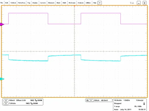
endix A. However, the next equations are added. manner. Therefore, the battery current is chopped during discharging using an IGBT at a very low frequency [12]. At the end of the off-period, the open circuit voltage is measured. The battery voltage waveform is monitored and analyzed to extract the other parameters at fixed SOC and temperature [14]. The measured current and corresponding voltage obtained by Yokogawa oscillo-scope for 55 A is shown in Figure 7. For better accuracy,

Tektronix DP07354 oscilloscope is used to measure the chosen cell voltage as depicted in Figure 8.

In modeling the battery, state of charge (SOC) is portant parameter to be determined. SOC relates the remaining capacity in Ampere-hour (Ah) to the con-sumed capacity [3,7,15]. For deriving the SOC, let Qobe

the initial capacity and Qn is the rated capacity. Hence,

the available or remaining capacity in Ah designated as

Qs and battery SOC are given as in Equations (1) and (2)

respectively.

SOCQ QS n. (2)

where, is is the battery current. The battery



C . (3)





internal vol- tage Eoc and terminal voltage Vt are given in Equations (3)

and (4) in terms of battery SOC and internal impedance respectively. The symbol (//) in Equation (4) stands for the parallel connection of the electric elements of the corresponding RC network.



trans1/ / trans1 t

t oc s bs

V E  i R R C 

3. Examination with TSLFP160AHA

To find all the parameters in the proposed model, an

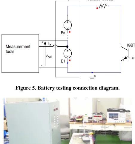
ex-Figure 5. Battery testing connection diagram. perimental battery test system was set up. The battery

bank is composed of 30 cells in series. One cell is chosen and its terminal voltage and current are measured as il-lustrated in Figure 5. The test is done at room

tempera-ture. Figure 6 shows the test system workplace. The ope-

rating conditions such as temperature, current and cycle number are kept close to each other. The battery open circuit voltage or internal voltage (Eoc) has a strong

rela-tionship with battery SOC [15]. The main target is to find this relation so that the battery SOC and hence the

re-maining capacity in Ah can be estimated with an accurate Figure 6. Battery test workplace.

ent waveforms seen by Yokogawa oscilloscope fo 55 A.

Figure 8. Voltage signals seen by Tektronix DP07354 oscilloscope for 55 A. The parameters in the proposed model are functions of

SO

ffect of current is small especially at higher cur-re

ohms of the vertical axis as shown from Figures 10 and

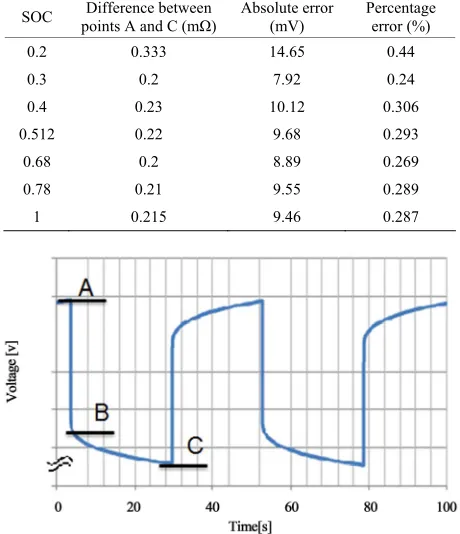
C, current, temperature and cycle number. However, the next tests show that the small error tolerance allows the parameters to be simplified or be independent of some variables. To consider the effect of current upon the battery parameters performance, the voltage differ-ence between the points A and B together and points A and C is measured and referred to current as illustrated in

Figure 9. The difference in voltage referred to current

between A and B represents the battery series resistance (Rbs) in Figure 3 while the difference between A and C

represents the whole battery impedance. Generally, the actual electric current demand of the electric vehicle var-ies according to the operating mode such as accelerating, constant speed or decelerating mode. The battery pa-rameters determination may vary according to the dis-charge current. Therefore, several currents are tested while the other variables are kept fixed. The percentage error evaluation is calculated within the tested current limits.

The e

nts. This is indicated from the close values in milli-

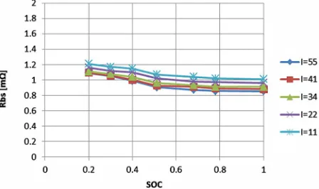
11. For fixed SOC, the vertical differences in Figures 10

and 11 are in the ranges of micro-ohms or fractions of

milli-ohm. For instance, considering that SOC equals 1, the vertical difference from Figure 11 between 11 A and

55 A is 0.215 mΩ. Of which about 0.156 mΩ relates to the battery series resistance (Rbs) as in Figure 10. This

will be translated into errors in ranges of milli-volts at the battery terminals. This would imply that between 11 A and 55 A, the battery terminal voltage error will be 9.46 mV (44 A × 0.215/1000). If this value is referred to 3.3 V from Table 1, then the error evaluation will be

0.287% (100 × 9.46 mV/3.3). The estimated error dif-ference between 11 A and 55 A for various SOC values is given in Table 2. This indicates that the parameters are

approximately independent of the discharging currents. Also at higher values of battery SOC as in Figures 10

and 11, the corresponding values of the impedances are

approximately fixed for a specified current. This current characteristics behavior simplifies the modeling proce-dures. The effect of current upon the individual parame-ters will be checked in the next section.

Table 2. Percentage error evaluation due to current variation.

Difference between Absolute erro

SOC _{points A and C (mΩ) (mV)} r Percentage _{error (%)}

0.2 0.333 14.65 0.44

0.3 0.2 7.92 0.24

0.4 0.23 10.12 0.306

0

0

.512 0.22 9.68 0.293

0.68 0.2 8.89 0.269

0.78 0.21 9.55 0.289

1 .215 9.46 0.287

Figure 9. Typical battery response waveform.

Figure 10. Measured voltage difference between A and B referred to current.

Figure 11. Measured voltage difference between A and C referred to current.

atic type battery having the same sp

ce

ance. Moreover in [1], it is referred that the capacity tests done with a prism

ecifications as the battery examined in this section showed that the tested cells still had a full capacity after 50 cycles. Also for repetitively or frequently used batte- ries, the monthly self-discharge can be ignored.

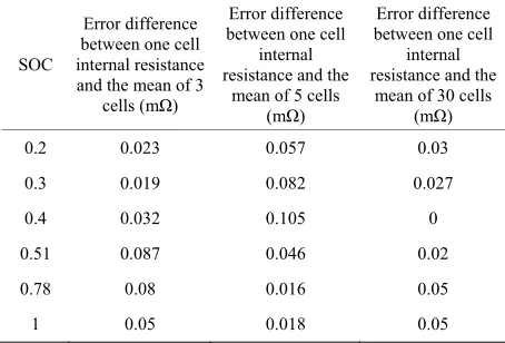
While stacking, the experimented battery bank cells are placed in series. To consider this effect of stacking on the battery bank, the battery internal resistance is calcu-lated for the chosen cell, three series cells, five cells and total number of cells in the bank. These numbers are chosen to decrease the error in measurements and calcu-lations. The analytical method used to calculate the bat-tery internal resistance is explained in Appendix A for one cell. The method is expanded for the series con-nected cells. The results are shown in Table 3. Consi-

dering a specific current, it was found that the mean values of the battery internal resistance Rbs of the series

con-nected cells are close to each other. As the actual power demand of EV varies with the operating mode, therefore a dynamic current of 55 A, which is close to the actual discharge current, is selected to calculate the battery in-ternal resistances. For instance with SOC equals 1, the error difference between one cell and the mean of three cells is 0.05 mΩ. The first cell terminal voltage error difference with respect to the mean value of the three cells will be 2.75 mV (0.05 mΩ × 55 A). Considering the mean values of the battery internal resistance per SOC value of the figures of Table 3 and the error differences between

the mean values and the chosen cell internal resistance, which are given in Table 4, it can be concluded that the

battery cells characteristics are very close to each other. Such characteristics of this prismatic type LiFePO4 battery simplify the modeling procedures. Therefore, one

ll is used to extract the model and its model will be applied to other cells from the same manufacturer.

Table 3. Effect of staking on the battery internal resist

Rbs for 55 A (mΩ) SOC

One cell Three cells Five cells 30 cells

0.2 1.084 _{Mean = 1.061}3.183 _{Mean = 1.027}5.133 _{Mean = 1.05}31.64 ₄

0.3 1.052 _{Mean = 1.033} 3.1 _{Mean = 0.97} 4.85 _{Mean = 1.025}30.75

0.4 0.95 _{Mean = 0.982} 2.9464 _{Mean = 0.845} 4.225 _{Mean = 0.95}28.57

0.51 0.89 _{Mean = 0.977} 2.9324 _{Mean = 0.844} 4.22 _{Mean = 0.91}27.23

0.78 0.86 _{Mean = 0.94} 2.82 _{Mean = 0.844} 4.22 _{Mean = 0.91}27.18

1 0.86 _{Mean = 0.91} 2.73 _{Mean = 0.842} 4.21 _{Mean = 0.91}27.17

EPE Table 4. Absolute value of the internal resistance error

dif-fe etween one cell and the mean of 3, 5 and 30 cells in series

SOC

E ffer be on inte and

rror diffe

e Error dt ce

nce and the

rence b .

rror di

tween e cell ence betwe_internal E

rnal resistance

the mean of 3 resistance and the resista rence

n one cell beween one cell ifferen internal

cells (mΩ) mean of 5 cells _(mΩ) mean of 30 cells_(mΩ)

0.2 0.023 0.057 0.03

0.3 0.019 0.4 0.78 0.082 0.105 0.046 0.027 0 0.02 0.032 0.087 0.08 0.51

0.016 0.05

1 0.05 0.018 0.05

Figure 12. Effect of current upon the open circuit voltage. Table 5. Battery open circuit voltage verus SOC at 55 A.

SOC Measured voltage (V) 0.18 3.0936

4. Model Extraction

In ral, O cuit volta ies accordi SOC,

tem a portant to he

nonlinear relation between th n circuit voltage and SOC for complete modeling. ambient t rature degrees are kept close to each other. For each SOC point,

voltage can take

0.2 3. 0.3 3.

129 1569 0.4 3.2352

gene pen cir ge var ng to

perature nd current. It is im e ope

find t

The empe 0.

0. 0. 51 3.275 68 3. 78 3. 2764 2622 0.85 3.27 0.88 3.290 0.93 3.3 0.96 3. 1 3. 367 38

the measurement of the open circuit

days. However, the effect of current upon the open cir-cuit voltage (Eoc), which is the voltage at point A of Fig-ure 9, is checked first for the same SOC points of Fig-ures 10 and 11. The results are illustrated in Figure 12.

Small open circuit voltage differences among the dis-charge currents indicate that the open circuit voltage is approximately independent of the tested discharge cur-rents. Therefore, the dynamic current will be tested care-fully at very high and very low SOC values in order to extract the open circuit voltage as a function of SOC.

For several days, the chosen cell open circuit voltage is measured at different SOC values and the fixed dy-namic current as shown in Table 5. The temperature of

the battery measured by the production company BMS is similar to the ambient in all readings. The temperature readings are 26˚C for all readings except for SOC equals 0.78, in which the temperature is 27˚C. For SOC low

Table 6. Percen error between m ed and fitted vol- tage.

Measured Fitted Absolute error Percentage

tage easur

SOC _{voltage (V) voltage (V) (mV) error (%)}

0.18 3.0936 3.1024 8.8 0.2844

0.2 3.129 3.1569 3.1605 3.2191 31.5 62.2 1.1 1.97 0.3 0.

0. 22. 0.

0. 0.

0.

3. 0.

3. 0. 0.

0.4 3.2352 3.2302 5 0.1545

51 68 3.275 3. 3.2764 3. 239 2535 36 54 1.09 697

78 3.2622 3.2618 33 0.01

0.85 3.27 3.267 3 0.09

0.88 3.29 3.27 0.02 0.6

0.93 0.96 3.3 3. 367 3. 274 315 026 052 0.78 1.54

1 3.38 352 028 83

er than 0.3, the battery open circuit voltage decreases expo- nentially. For medium and high values of SOC, the open circuit voltage increases linearly with small slope. For very high values of SOC, the open circuit voltage in- creases with some non-linearity in the measured voltage. The next function given in Equation (5) is used to fit the empirical data of Table 5. Table 6 gives percenttage

error between the fitted values and the measured data.

11SOC

2 0.92e 3.197 0.188SOC 3.197 0.08317SOC for 0.3 SOC

oc E      _   

2_0.3 3 _for

0.0 SOC 2SOC SOC

1.018SOC for SOC 0.95

         (5)

999 0.3

0.95 

3.4 1.06583SOC

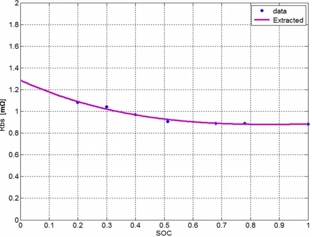
Considering the experimental tests of Section 3, The RC networks values as functions of SOC can be ex-tracted. Figure 10 directly represents the battery internal

resistance (Rbs). It is redrawn in Figure 13 with SOC in

the x-axis. The method used to find the parameters of the attery is explained in Appendix A for fixed SOC and b

temperature. Figures 14-17 represent the short term and

long term time constants resistances and capacitances. Away from the long term time constant capacitance,

Figure 16. Long term time constant resistance as a function of SOC.

Figure 13. Battery internal resistance as a function of SOC.

Figure 17. Long term time constant capacitance as a func-tion of SOC.

current has very slight effect on the parameter determina-tion. Therefore, a dynamic current for the electric power demand close to the actual discharge current should be

ven though averaging technique can be used for e long term time constant capacitance, however the error evaluation of the currents close to the dynamic cur-rent will be checked in the next section to prove the va-lidity of the single variable curves. Moreover by investi-gating Figures 13-17, the parameter values of the

cur-rents near the dynamic current are very close to each other. From Figures 18 to 22, the calculated values from

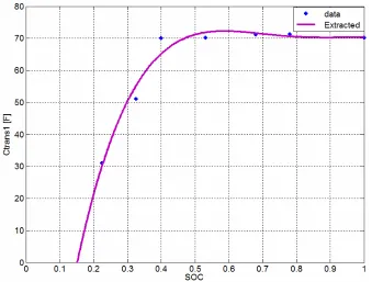
measurements are drawn by an asterisk and the best-fit-ted curves are drawn by a continuous red color. All the extracted parameters are fixed in the region from 40% to 100% SOC. Using the curve fitting method to these em-pirical data, the following functions are used to represent these curves:

Figure 14. Short term time constant resistance as a function of SOC.

selected to extract the parameters to find single-variable curves. E

th





bs

R     (6)

Figure 15. Short term time constant capacitance as a func-tion of SOC.





trans1

3 4

SOC 2 10.554SOC 22.604SOC 20.59SOC 7.1067SOC

R   





3 4

SOC 110 940SOC 1800SOC 1500SOC 460SOC

C    

  (8)





trans2

3 4

SOC 0.13 0.28SOC+0.6SOC 0.56SOC +0.19SOC

R  

 (9)









3 4

SOC 9.19 1020.3SOC 1829.7SOC

1361.2SOC 354.54SOC 1000

C    

   (10)

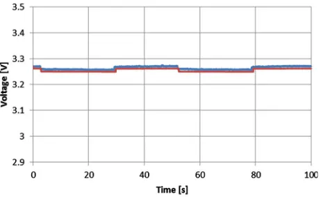
In order to check the voltage behavior of the extracted model during the rest time, the simulated results ing to Equations from (5) to (10) and the corresponding experimental results are shown from Figures 23 to 27 for

SOC equals 0.78. The rest time is the time corresp to the off-period. Even though the model is extracted at the dynamic current, however the close agreement be-tween the experimental and simulated results proves the above equations can be used during the rest tim describe the battery behavior.

accord-onding

that e to

Figure 18. Extracted battery internal resistance.

Figure 19. Extracted short term time constant resistance.

Figure 20. Extracted short term time constant capacitance.

Figure 21. Extracted long term time constant resistance. From the experiments done with LFP battery and

ex-tracted parameters, some observations are found. First, all the resistive elements increase with SOC lower than 0.4. Also, all the capacitive elements decrease with SOC lower than 0.4. This means when the battery near flat, its resistive elements are more dominant than capacitive

parameters and hence it will be sensitive for the dis-charging currents. The battery internal resistance Rbs is

Figure 22. Extracted long term time constant capacitance.

Figure 25. Voltage profile with SOC = 0.78 and I = 34 A [Blue: experimental, red: simulated].

and I = 55 A Figure 23. Voltage profile with SOC = 0.78

[Blue: experimental, red: simulated].

Figure 26. Voltage profile with SOC = 0.78 and I = 22 A [Blue: experimental, red: simulated].

and I = 41 A Figure 24. Voltage profile with SOC = 0.78

[Blue: experimental, red: simulated].

Figure 27. Voltage profile with SOC = 0.78 and I = 11 A [Blue: experimental, red: simulated].

(a)

(b)

igure 28. The Voltage drop across R F

SOC = 0.78 (

bs versus current with

experimental results) [(a): 55 A, (b): 22 A]. constant can be related to the capacitance, which is re-lated to the permittivity between the two electrodes. This observation comes as a result of the short term time con-stant capacitance value, which is affected by SOC rather than current. Long term time constant appears to describe the electrochemical reactions in the electrolyte behavior. This is because its related capacitance is affected by the

OC. In general, the long term time constant capacitance decreases with reducing the discharging current [12].

5. Model Validation and Discussion

After experimentation procedures with TSLFP160AHA bank, the battery is left about 24 hours. The correspond-ing voltage after that time is called the rest voltage as illustrated in Figure 29. It is observed that the voltage at

point A1 (in the first off-period) is lower than the rest voltage. This voltage difference appears to be caused as an effect of current. This overcharge phenomenon is rep-resented by ( e

discharging current and S

s i t



 ) as an addition to Equation (5), in which α is the difference between the rest voltage an

under any operating condition than 0.025 V and β is set to 0.0003 to imitate the drop in the voltage profile respectively. This effect is not common in the next off periods after the point A1. Therefore, it can be neglected because it does not affect battery steady state or long term operating performance.

ANSOFT SIMPLORER is a good and simple tool to represent the equivalent circuit of the proposed model. It provides a ready block to implement the algebraic equa-tions directly and the outputs of these equaequa-tions deter-mine the electrical elements behavior. Moreover, it offers some blocks to implement the mathematical equations

nufacturer company, Equations from (5) to (10) are considered general func-tions for high current healthy prismatic type cells of high power LFP batteries. In order to prove the generality of the extracted model, the GBSLFMP 60 Ah battery bank from the same production company is continuously dis-charged through a resistive load. From the datasheet of this battery, it has 60 Ah rated capacity. One cell is cho-sen and its voltage profile is recorded. The discharge test is done when the battery is fully charged up to its final state indicated by an alarm from the BMS system. All the recognized parameters extracted from TSLFP160AHA bank are directly applied to GBSLFMP 60 Ah battery bank. Figure 30 shows the experimental results for 1 C

discharging. The same data is compared with the simu-lated results in Figure 31. o investigate the

ac-curacy of Figure 31, a zoomed in image is drawn in

Figure 32. The maximum operating time error between

the simulated and experimental results is 50 mV with 1.7% referred to the experimental value and takes place in the exponential zone. Table 7 gives the different

ac-curacy values for different current ranges, which proves the validity of the model. It should be noted that the op-erating time error percentage in Table 7 is the absolute

d point A1 in Figure 29 and β is an adaptive parameter.

The value of α does not increase

that include differentiation or integration.

Considering discharging currents close to the dynamic urrent, at least for the same ma

c

Copyright © 2012 SciRes. EPE nd effect of current.

Figure 29. Rest voltage a

Figure 31. Voltage profile with GBSLFMP 60 AH for 1 C discharging [Blue: experimental, red: simulated].

Figure 32. Zoomed in image of the voltage profile with GBSLFMP 60 AH for 1 C discharging [Blue: experimenta d: simu-lated].

Copyright © 2012 SciRes. EPE o the experimental values.

The difference occurring in the exponential region in-dicates that cell resistances are lower than the extracted values at that region. This would imply that this cell is healthier than other cells in the bank. It can work for ex-tra time or exex-tra Ahs compared with the cell that gives an alarm. During testing, temperature varies from 26˚C to 30˚C indicating that this temperature difference has neg-ligible effect on the battery performance.

For more comparison, Figure 33 shows a zoomed in

image of the simulated and experimental results of a 0.5 C continuous discharging current. The maximum operat-ing time error for 0.5 C occurs at the beginnoperat-ing of the exponential zone. Also, the maximum operating time error for 0.3 C occurs at the beginning of the exponential zone as shown in Figure 34. For 1 C, 0.5 C and 0.3 C

discharging currents, the error during the linear region is small. However, when the battery is discharged at 2 C as in Figure 35, there is a long period operating time error

of 45 mV during the linear region. This error is because 2 C discharging current is far from the dynamic current at which parameters equations are extracted. Also, there was an alarm occurred many times that makes the charging to be stopped. The interruptions during the dis-charging with 2 C indicate that there is at least one cell inside the battery bank gave an alarm. This implies that the small error tolerances between the individual cells become

Regarding the authors’ applications, there is a 30 KW vehicle under construction in KERI laboratory. The bat-tery bank used in this vehicle is not used to receive

re-supercapacitor module will be used to recover such ener- gy. Therefore, this paper focuses on the discharging mode to determine the area or SOC value at which the battery is working. During charging, the GBSLFMP 60 Ah battery bank was charged with constant current in a separate utility. The BMS gives an alarm if any cell ter-minal voltage increases 3.6 V. Figure 36 shows the

ter-minal voltage of the battery bank during charging with 1 C and discharging with 1 C and 0.5 C. Unfortunately, during charging, the battery open circuit voltage does not follow Equation (5). The effect of current appears strongly at the battery terminal voltage. There is a long non-linear zone at the beginning. Also, the overcharge region is non-linear. Even at the linear region, the mea- sured terminal voltage is higher than the calculated. Therefore, two-dimensional look-up table with interpola-tion can be implemented in ANSOFT SIMPLORER to represent the terminal voltage charging profile with SOC or time and Equation (4) can be used to determine the battery open circuit voltage.

6. Conclusion

This paper proposes an accurate modeling of lith-ium-iron-phosphate battery (LFP) battery. The model includes six parameters measured by an experimental manner as a function of SOC. The experimental results e same production company. The battery parameters are fixed as SOC varies from 40% to 100%. The battery current has slight effect on the battery parameters. The effect of value of the difference between the experimental and

simulated values referred t

generative energy during vehicle operation. Instead, a

large at higher currents. are carried out with two different batteries from th

r 0.3 C red: simulated]. Figure 34. Voltage profile with GBSLFMP 60 AH fo discharging [Blue: experimental,

Copyright © 2012 SciRes. EPE Figure 36. Measured terminal voltage profile with GBSLFMP 60 Ah bank [Brown: 1 C charging, green: 1 C discharging, blue: 0.5 C discharging].

Figure 37. Analytical approximation of battery terminal voltage response due to a current pulse. Table 7. Voltage error comparison results.

Current Maximum error _{voltage (mV)} Operating time error (%)

stacking is discussed in this paper. The battery has three regions: exponential, linear and non-line

voltage ar. The close agreement between the simulated and measured data indicates that the model can predict the battery per-formance to within 1.7% operating time error. For given battery terminal voltage and discharge current, especially during the linear region as the accuracy is very high, bat-tery open circuit voltage can be estimated. Therefore, the model can be used to predict battery SOC. The model

2 C 45 1.48%

1 C 50 1.7%

0.5 C 10 0.3%

can be easily repeated and modified for different battery technologies and can be extended for wide dynamic ranges of different currents. In all, the model offers cir-cuit and system engineers the possibility to improve the efficiency and size the LFP battery for automotive appli-cations by predicting both the battery performance and I-V characteristics with co-simulation in ANSOFT SIMPLORER.

REFERENCES

[1] F. P. Tredeau and Z. M. salameh, “Evaluation of Lithium Iron Phosphate Vehicles for Electric Vehicle Applica- tion,” IEEE Vehicle Power and Propulsion Conference, Dearborn, 7-10 September 2009, pp. 1266-1270.

[2] E. J. William, et al., “A Comparative Study of Lithium Poly-Carbon Monoflouride (Li/CFx) and Lithium Iron Phosphate (LiFePO4) Battery Chemistries for State of Charge Indicator Design,” IEEE International Symposium on Industrial Electronics, Seoul, 5-8 July 2009, pp. 2006- 2009.

[3] C. H. Cai, D. Du, J. T. Ge, Z. Y. Liu and H. Zhang, “Bat-tery-Charging Model to Study Transient Dynamics of Battery at High Frequency,” IEEE Region 10 Conference on Computers, Communications, Control and Power En-gineering, 28-31 October 2002, pp. 1843-1846.

[4] J. M. Miller, “Energy Storage System Technology Chal-leng

Veh

ence, Dearborn, 7-10 September 2009, pp. 4-10.

[5] J. Larminie and J. Lowry, “Electric Vehicle Technology Explained,” John Wiley & Sons, Ltd., Chichester, 2003. [6] H.-S. Kim, “Secondary Battery and Material,” Korea

Electrotechnology Research Institute (KERI) Lectures, June 2010, p. 17.

[7] P. Thounthong, V. Chunkag, P. Sethakul, B. Davat and M. Hinaje, “Comparative Study of Fuel-Cell Vehicle Hy-bridization with Battery or Supercapacitor Storage De-vice,” IEEE Transactions on Vehicular Technology, Vol.

58, No. 8, 2009, pp. 3892-3904. doi:10.1109/TVT.2009.2028571

[8] C. S. Edrington, O. Vodyakho and B. A. Hacker, “De- velopment of a Unified Research Platform for Plug-In Hybrid Electrical Vehicle Integration Analysis Utilizing the Power Hardware-in-the-Loop Concept,” Journal of Power Electronics (JPE), Vol. 11, No. 4, 2011, pp. 471-478. doi:10.6113/JPE.2011.11.4.471

[9] J. Bauman and M. Kazerani, “A Comparative Study of Fuel-Cell-Battery, Fuel-Cell-Ultracapacitor and Fuel-Cell- Battery-Ultracapacitor Vehicles,” IEEE Transactions on Vehicular Technology, Vol. 57, No. 2, 2008, pp. 760-769. doi:10.1109/TVT.2007.906379

[10] M. Ziyad, M. A. Salameh, W. A. Casacca and Lynch, “A Mathematical Model for Lead-Acid Batteries,” IEEE Transactions on Energy Conversion, Vol. 7, No. 1, 1992, pp. 93-98.

[11] Y. Kim and H. Ha, “Design of Interface Circuits with Electrical Battery Models,” IEEE Transactions on Indus- trial Electronics, Vol. 44, No. 1, 1997, pp. 81-86. [12] K. S. Champlin and K. Bertness, “A Fundamentally New

Approach to Battery Performance Analysis Using DFRATM_/DFISTM _{Technology,” 22nd International Tele-}

communications Energy Conference, Phoenix, 10-14 Sep- tember 2000, pp. 1-6.

[13] M. Chen and G. A. Ricon-Mora, “Accurate Electrical Battery Model Capable of Predicting Runt e and I-V Performance,” IEEE Transactions on Energ nversion,

[14] B. Schweighofer, K. M. Raab and G. Brasseur, “Model-ing of High Power Automotive Batteries by the Use of an Automated Test System,” IEEE Transactions on Instru-mentation and Measurement, Vol. 52, No. 4, 2003, pp. 1087-1091. doi:10.1109/TIM.2003.814827

es Facing Strong Hybrid, Plug-In and Battery Electric icles,” IEEE Vehicle Power and Propulsion

Confer-im

y Co

Vol. 21, No. 2, 2006, pp. 504-511.

[15] A. Szumanowski and Y. Chang, “Battery Management System Based on Battery Nonlinear Dynamics Model-ing,” IEEE Transactions on Vehicular Technology, Vol. 57, No. 3, 2008, pp. 1425-1432.

doi:10.1109/TVT.2007.912176

Appendix A

The determination of the equivalent circuit model pa-rameters for constant SOC and temperature can be ob-tained by investigating the battery terminal voltage pro-file of a current pulse as shown in Figure 37. The

inter-nal resistance and the short term time constant can be

tion of the resulting waveform can be approximated to Equation (11). The designation t

and v(t) corresponds to the time and terminal voltage respectively. Hence, the battery internal resistance (Rbs),

short term constant resistance (Rtrans1) and short term

constant capacitance (Ctrans1) can be obtained according to Equations (12)-(14). Investigating the remaining part of the waveform, the long term time constant parameters can be obtained in a similar manner.

defined by investigating the first 0.5 s of the terminal voltage profile. The solu

 





trans1 1 e

oc R

v t E _V V  _. (11)

bs R

R V I . (12)

trans1 trans1

R V I. (13)

trans1 trans1 trans1