Forecasting of wind power production in the Netherlands

Forecasting of wind power production in the

Netherlands

THESIS

by

Yme Joustra

Master of Science in Computer Science

University of Twente, the Netherlands

August 26, 2014

Preface

After working for several years at Raedthuys Pure Energie, it became clear how interesting the renewable energy industry is. Searching for interesting areas in the energy world is not hard (since there are plenty), but to create a decent sci-entific research of it is. Combining my interest in the area of machine learning with the possibility of performing a research at Raedthuys narrowed the amount of areas down to a few certain areas in the field of forecasting wind power. At the company I mainly focus on the analysis of producing wind power. During this analysis the company noticed that the forecasting methods they used did not perform as well as they expected. The challenge finding a suitable forecast-ing technique for day-ahead wind power predictions motivated me to conduct research in this area.

I would like to thank Maurice van Keulen and Mannes Poel, my supervisors from the University of Twente for guiding me through the process of this research and for providing me feedback. I would also thank Dolf Trieschnigg for his guidance and feedback during the literature study part of this research.

Furthermore, I would like to thank Martijn Tielkes and Erik Veer, my su-pervisors from Raedthuys for guiding me through the process of wind power forecasting and for helping me to understand the energy market in detail. I have learned many things during my research.

Finally, I would like to thank my fellow students, my best friends and es-pecially my girlfriend for supporting me during the past few months, for their feedback and useful discussions on the subject.

Abstract

Wind power has become an important source of power for some countries be-cause wind is renewable, wind power is clean and no pollutants are produced compared to fossil fuels which are mainly used for the generation of energy to-day. Because of these reasons also in the Netherlands attention towards the use of wind power has grown. In the past decade, a lot of research has been performed on the forecasting of wind power production over a period of min-utes, days, months and years. This paper focuses on day-ahead forecasting and starts with a theoretical and economical overview of the electrical grid and en-ergy market. The main reasons to focus day-ahead forecasting is to ensure the balance between the demand and supply of electricity and because the energy needs to be sold against a day-ahead spot price. Based on a literature study in the field of forecasting wind power it has been found that factors such as geo-graphical location, data sources and grid sizes show influence on the accuracy of the data and therefore influence the prediction of wind power. Furthermore, based on the literature input parameters such as wind speed, wind direction, weather stability, availability, relative humidity and seasonal data have been found useful as input data for forecasting methods to forecast wind power day-ahead. From a large set of forecasting methods it has been found that the most used techniques to predict wind power day-ahead are physical methods, and statistical or hybrid methods such as neural networks.

This research has obtained forecasting results from a Random forest, Feed forward neural network and a hybrid model consisting of a combination of un-supervised k-nearest neighbour clustering and a neural network. These results have been compared with the forecasting results obtained from an external or-ganization. Based on the comparison of monthly and average monthly MAPD and RMSPD we have found that the Feed forward neural network and the hy-brid model are able to obtain a performance equally or even better compared to the external forecasting for a single turbine. The input parameters that made the difference were the u-vector, v-vector, the use of SCADA data and the wind speed time lag 1.

Glossary

Electrical grid: The grid through which electricity is being transmitted.

TSO: Transmission System Operator who is keeping the balance between sup-ply and demand of electricity on country level.

DSO: Distributed System Operator who is keeping the balance between supply and demand of electricity on region level.

Energy trader: Is responsible for optimising the production and supply fore-cast by buying and selling electricity on the wholesale trading market.

PR: Program Responsible is responsible for informing the TSO based on the most actual forecast and trading position in order to support the balance between demand and supply.

Short: There is being less energy produced than forecasted. In other words an underproduction.

Long: There is being more energy produced than forecasted. In other words an overproduction.

APX: A day ahead (or spot) market price based on submitted orders of demand and supply of electricity on a hourly basis.

Helper: A producer whose portfolio is short when the TSO is long or whose portfolio is long when the TSO is short.

Causer: A producer whose portfolio is short when the TSO is short or whose portfolio is long when the TSO is long.

Imbalance: The difference between the forecasted amount and the allocated amount of energy produced.

NWP: Numerical weather predictions (NWP) are based on the current weather conditions of the atmosphere and are calculated using models. Numeri-cal means that each data value is represented as a number (a series of numbers).

Contents

1 Introduction 1

2 Background 3

2.1 Infrastructure of the electrical grid . . . 3

2.2 Parties and their roles in the energy market . . . 4

2.2.1 Physical flow . . . 5

2.2.2 Information flow . . . 6

2.2.3 Cash flow . . . 6

2.2.4 Horizontal dashed line . . . 7

3 The importance of forecasting 7 3.1 Balancing demand and supply . . . 7

3.2 Economic perspective . . . 8

3.2.0.1 Scenario 1 -Pt>0 andPt< Pa : . . . 9

3.2.0.2 Scenario 2 -Pt>0 andPt> Pa: . . . 10

3.2.0.3 Scenario 3 -Pt<0: . . . 10

3.3 Discussion . . . 11

4 Introduction to forecasting models 12 4.1 Random forest model . . . 12

4.1.1 Process of the Random Forest . . . 12

4.2 Feed forward Neural Network . . . 13

4.2.1 Process of the feed forward neural network . . . 13

4.2.2 Learning the algorithm . . . 14

4.2.3 Hidden neurons and layers . . . 14

5 Related work 14 5.1 Important factors for forecasting wind power . . . 15

5.1.1 Data sources . . . 15

5.1.2 Grid area . . . 16

5.1.3 Geographical location . . . 16

5.2 Input parameters for forecasting models . . . 17

5.2.1 Wind speed . . . 17

5.2.2 Wind direction . . . 18

5.2.3 Weather stability . . . 19

5.2.4 Availability . . . 19

5.2.5 Relative Humidity . . . 20

5.2.6 Seasonal . . . 20

5.2.7 Temperature and pressure . . . 21

5.3 Forecasting models . . . 21

5.3.1 Statistical models . . . 22

5.3.1.1 Regression trees . . . 22

5.3.1.2 Time series models . . . 22

5.3.1.3 Artificial Neural networks (ANN) . . . 23

5.3.1.4 Support vector regression/machine . . . 24

5.3.1.5 Discussion . . . 25

5.4 Feature selection methods . . . 26

6 Methodology 27

6.1 Data sources . . . 27

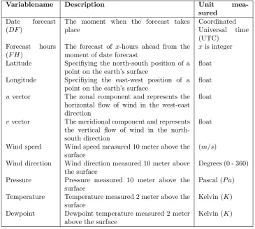
6.1.1 Data description . . . 28

6.1.2 Meteorological data . . . 28

6.1.3 SCADA data . . . 29

6.1.4 Production data . . . 29

6.1.5 Data tools . . . 31

6.2 Methods of analysing data . . . 31

6.3 Training, validation and testing forecasting models . . . 32

6.4 Performance measurements . . . 33

7 A hybrid model 34 7.1 Step 1: Unsupervised k-nearest neighbor clustering . . . 34

7.1.1 Process of the algorithm . . . 34

7.1.2 Applying unsupervised k-nearest neighbor clustering al-gorithm . . . 35

7.2 Step 2: Applying feed forward neural network . . . 36

8 Data analysis 37 8.1 Grid point reduction . . . 37

8.2 Selection of input features . . . 38

8.3 Correlation studies . . . 39

8.3.1 Correlation coefficient . . . 39

8.3.2 Discussion . . . 40

8.3.3 Autocorrelation coefficient . . . 45

8.4 Cook’s distance measure . . . 46

8.5 Scada data and wind speed distribution analysis . . . 46

8.6 Conclusion . . . 48

9 Results 49 9.1 Single turbine . . . 51

9.2 Wind farm of 27 Turbines . . . 53

9.3 34 Turbines . . . 54

9.4 Financial impact of one turbine . . . 55

10 Discussion 56 10.1 Single turbine . . . 56

10.2 Wind farm of 27 turbines . . . 58

10.3 34 Turbines . . . 60

10.4 Input parameters . . . 60

11 Conclusion 62

1

Introduction

Consumers have become accustomed to a stable electricity supply. This electri-cal supply is produced using different sources such as burning fossil fuels, using solar panels or wind turbines. This research will focus on energy used for the electricity supply which is produced by wind turbines. This form of energy is also called wind power. A major difference between wind power and fossil fuel energy is the predictability of producing energy. A predictable source can be used to balance the supply to the demands. Balancing the demand and supply of electricity is important to ensure continuous electricity supply. For instance one expects to start one’s computer when one puts the plug into the socket. Fossil fuels such as gas differ from wind power in terms of predictability, as is indicated below:

Predictability - Fossil fuels (gas): Energy can be produced by a fossil fuel such as gas. Fossil fuels have a limited capacity and are in stock. Therefore the production of energy is predictable.

Predictability - wind: Energy can also be produced by wind turbines. How-ever wind is unpredictable and therefore one cannot ensure the availability of wind power when needed. In other words: one cannot rely on producing energy using wind if one cannot predict this source.

The predictability of wind power production is therefore a major drawback, because one cannot ensure the availability of wind power when needed. How-ever, compared to fossil fuels, wind has its advantages; there is plenty of wind available, wind is renewable, wind power is clean and no pollutants are pro-duced.

Using only energy produced by wind turbines is not yet possible since no country is able to provide enough wind power to ensure a continuously electricity supply. The Netherlands for instance, produced only 4.9% wind power by wind turbines of its total electricity consumption in 2012 [6].

Therefore nowadays the supply of electricity is based on the production of both forms of energy, fossil and renewable. However an issue arises using this combination, giving a scenario.

Scenario - combination: Energy will be produced by fossil fuels and wind turbines. Since wind is a variable source one does not know how much energy is produced by wind turbines. This makes it difficult to keep the balance between demand and supply of energy, because one does not know how much fossil fuels to use to keep this balance.

Clearly, it is difficult to keep the balance between the demand and supply of energy when at least one energy source is uncontrollable, which is addressed by Soman et al. [43]. A solution to deal with the uncontrollability of renewable energy is the use of accurate forecasting techniques to predict the production of energy by these sources. Forecasting techniques provide forecasts about the amount of wind power produced by wind turbines.

focus on a time scale called day-ahead (24 to 48 hours) forecasting. The reason focusing on this time scale is because regulators of the net; like the Transmission System Operator (TSO) and the Distributed System Operators (DSO), need to know how much wind power will be produced day-ahead so they can ensure the balance between the demand and supply of electricity. Using these forecasts regulators can respond easier on balancing the demand and supply of electricity, because now the amount of wind power generated by turbines does not come as a surprise.

Another reason focusing this time scale day-ahead is because the energy needs to be sold against a day-ahead spot price. Both reasons are discussed in more detail in section 3.

A lot of research in the field of forecasting wind power has been performed. Literature overviews (e.g. [27],[49]) have identified different prediction models for different time scales in different countries. Also research has been conducted to find the right input parameters that influence the outcome of the prediction model. The amount of different prediction models and the use of factors in literature studies lead to the following research questions:

RQ1 Which factors and input parameters to predict wind power have been described in literature? And which of those have been found successful?

RQ2 Which forecasting models have been found the most relevant by previous literature to predict wind power generated by wind turbines?

These first two research questions are answered performing a literature study which is given in section 5. Determining which factors and input parameters have been found successful is based on what literature recommends to use to predict wind power. If parameters increase the accuracy of the prediction model they will be found successful and the other way around.

Besides the literature study, this research will be conducted at the company Raedthuys Energie BV. Since more attention is given to renewable energy in the Netherlands, more research in the field of forecasting wind power generated by turbines can be conducted, specifically in the Netherlands.

Raedthuys Energie BV, located in Enschede, is a renewable energy producer in the Netherlands. About 50 employees are working at Raedthuys. Their mission is to stimulate the use of renewable energy and the goal is the delivery of sustainable energy from wind and sun to its customers using wind turbines and solar panels. Raedthuys earns his money by realizing a large set of activities which are developing, investing, building, managing and ensuring renewable energy projects and the delivery of renewable energy [38].

Forecasting wind power is important for Raedthuys because they sell their forecasted energy day-ahead. It is a ‘risk’ to sell the production of energy real-time, which will be explained in section 3.2. It is therefore important to have a model that can forecast wind power generated by wind turbines as accurate as possible. Currently Raedthuys is using forecasts of wind power provided by external organizations. However they want to have their own forecasting model so they do not depend on other organizations. Therefore we have to build a forecasting model that performs at least equal to the current forecasts, which gives us the overall research questions of this research:

RQ4 Which input parameters and optimizations have to be applied on the rec-ommended forecasting models to achieve an as accurate prediction model compared to the forecasting model from the external organizations?

Identifying the input parameters mentioned in research question three is done using several correlation studies see also section 8. The input parameters are used to find the forecasting model that performs best.

The structure of this document is as follows. Section 2, explains the back-ground of the subject. Section 3 explains in detail the importance of forecasting wind power generated by wind turbines. Section 4 describes which forecast-ing techniques are used to predict wind power. Section 5 provides a literature overview about the subject. Section 6 describes the methodology of this re-search, what data and methods have been used and how they have been used. Section 7 describes our proposed hybrid model. Section 8, explains stepwise how data has been selected and extracted. Section 9 provides the results obtained by the different forecasting techniques with the right parameter estimation. Sec-tion 10 discusses the obtained results. SecSec-tion 11 presents the conclusion of this study. Finally, some future work is given in section 12.

2

Background

To understand the research questions and our related work 5 we explain the infrastructure of the electrical grid (section 2.1) and the energy market (sec-tion 2.2).

2.1

Infrastructure of the electrical grid

Figure 1 shows the infrastructure of the electrical grid in the Netherlands. As one can see, the figure presents different parties who are part of the grid. In this figure only renewable energy producers wind and solar have been taken into account. Other renewable energy sources such as hydro energy or biomass energy are not included in the picture because these are beyond the scope of this research.

Furthermore, the figure also presents different levels of electrical power trans-mission (the load transtrans-mission of electrical energy). Each of the load transmis-sion levels of electrical energy will be explained below:

220 - 380 kV: This is the top level of the electrical power transmission. The power plants produce a high voltage of electricity using fossil fuels. Using high voltages is because they can be transferred over large distances with less losses. The electricity is transferred via transmission lines. The load of electricity in the transmission lines is regulated by the Transmission System Operator (TSO), TenneT in the case of the Netherlands [45].

Figure 1: Infrastructure of the electrical grid (provided by Raedthuys Energie BV.)

connect turbines to the highest level of voltage. The electricity is trans-mitted to large consumers of electricity (e.g. industrial consumers) and Distributed System Operators (DSO). DSOs regulate the grid on a smaller (regional) area than the TSO does.

0.4 - 25 kV: The electricity transmission from the second level is converted by the DSO to a much lower voltage. This load of electricity is distributed to end users (e.g. household consumers) that belong to the area of the DSO. End users with solar panels produce electricity which flows into the grid or is consumed by the end user itself.

The TSO also collaborates with the other European TSOs to compensate electricity shortages and surpluses [45]. A discussion of the European market is beyond the scope of this research.

2.2

Parties and their roles in the energy market

Trader and the Program Responsible (PR). The job of the energy trader is to buy energy from the producers, sell energy to the suppliers and trade energy with other traders on the Energy trading market. The PR is responsible for informing the TSO based on the most actual forecast and trading position in order to support the balance between demand and supply. [9][46].

The edges show the flow between the parties. There are three types of flows visible in the figure, namely the physical flow on the grid (black lines (MWh)), the Information flow (Green lines (Info)) and the Cash flow (Red lines (e)). To understand the graph each flow will be described by explaining the edges.

The horizontal dashed line in the middle divides the picture into an energy market (upperside) and the electricity grid (underside). The upper side and underside always have to be balanced. More information about this line will be given in section 2.2.4.

Transmission System Operator

(TSO) Producer

Energy Trader / Portfolio Manager

---Program responsible (PR)

Distributed System Operator

(DSO)

Consumer Supplier

MWh Info

€

MWh

MWh

€

€

Info

€

Info

Info

Info Info

€

€

Energy market

Electricity grid

Figure 2: The structure of parties in the energy market

2.2.1 Physical flow

the other way around to ensure decentralized production of energy. The TSO and DSO both are independent companies. Their main job is to manage the balance between the demand and supply of electricity. The electrical grid is being balanced by regulating the amount of electricity through the electrical grid. To ensure the quality and continuous supply of electricity the grid needs to be maintained [34][45]. Maintaining the grid costs the TSO and DSO money. The difference between the TSO and DSO is that the TSO is managing the transport of electricity on the electrical grid on country level, whereas the DSO is managing the electrical grid on a specific region.

2.2.2 Information flow

The flow of information between parties consists of information about the fore-casted values to be produced and consumed and the actual values produced and consumed. For each of the parties the following information is being shared.

Producer →Energy trader: The producer informs the Energy trader about the forecasted amount of electricity produced for the next day.

Supplier →Energy trader: The supplier informs the Energy trader about the forecasted amount of electricity consumed by the consumers.

PR →TSO: The PR informs the TSO about its purchase and sale transac-tions of electricity. The PR tries to balance the demand and supply of electricity using the information from the supplier and the producer. To keep the balance the PR is responsible for buying and selling electricity on the market.

DSO →TSO: The DSO regulates the electricity grid real-time in its own re-gion and informs the TSO about the actual amount of electricity consumed by the consumers.

DSO →Supplier: The DSO informs the supplier about the actual amount of electricity consumed by the consumer.

TSO → PR: The TSO regulates the high voltage electricity load through the transmission lines real time and informs the PR about the actual amount of electricity produced and consumed.

2.2.3 Cash flow

In the cash flow a party buys or sells energy, settles imbalances or maintains the electrical grid. How the cash between parties flows is explained here:

Energy trader →producer: The Energy Trader pays the producer for sell-ing his amount of electricity.

Supplier →Energy trader: The supplier is responsible for buying electricity from the energy trader.

Supplier →DSO: The supplier pays the DSO for its services. These costs have already been paid by the consumer, since the consumer has paid the supplier for the DSO its services.

Producer ←→ PR: the difference between the forecasted amount and the al-located amount of electricity produced is called the imbalance and is fi-nancially settled. One has to pay the other depending on the so called imbalance price, which can be positive or negative.

Producer ←→ TSO: the difference between the forecasted amount and the allocated amount of electricity produced and consumed is called the im-balance and is financially settled. One has to pay the other depending on the so called imbalance price, which can be positive or negative.

2.2.4 Horizontal dashed line

The horizontal dashed line divides figure 2 into the energy market/cash flow (top) and the physical flow on the grid; the electricity grid (bottom). The cash flow represents the forecasted amount of energy bought and sold. This means in an ideal situation where the forecasts are 100% accurate, the cash flow of energy bought and sold represents the energy transmitted through the electrical grid. However since forecasts are never 100% accurate, there exists a difference between the forecasted and allocated amount of energy, which unbalances the demand and supply. This difference is also called the imbalance. To balance the demand and supply two extra cash flows have been added. One between the producer and PR and one between the PR and the TSO (underside of the figure). These cash flows are the settlement of the imbalance by the TSO and are required to ensure the balance between the demand and supply of energy in the overall cash flow as in the electricity flow.

The next section explains the importance of forecasting wind power, by discussing several scenarios to understand the energy market in practice.

3

The importance of forecasting

As mentioned in the previous section the demand and supply of energy needs to be balanced. This is the main reason using forecast energy. However there are also costs bound to these forecasts. These are the two cash flows between the producer and the PR and the PR and the TSO, see also figure 2. In this section we will explain the importance of forecasting wind power by discussing several scenarios. The first subsection discusses balancing the demand and supply of energy and the second subsection discusses the economic perspective of forecasting wind power.

3.1

Balancing demand and supply

TSO uses this information to regulate the electrical grid [45]. Without know-ing the predicted wind power issues will arise, because the TSO will use only fossil fuels for energy production. Issues such as regulating the grid to keep balance between the demand and supply of electricity can occur. Therefore the importance of knowing the predicted wind power gives the TSO the possibility to estimate the amount of fossil fuels needed to ensure the balance between demand and supply of energy. In other words to regulate the grid easier. When the actual wind power production is known the electrical grid isshortorlong. A grid being short means there is less wind power produced by the turbines than forecasted. In other words an under production. A grid being long is the other way around, an over production. The reason of this under or over production is because predictions are almost never 100% accurate. Actions taken when the electrical grid isshort orlong are explained in the following scenarios.

Scenario 1: There is a short on the electrical grid. The TSO needs to ramp up the energy by producing energy using the fossil fuel power plants to ensure the balance between demand and supply of energy.

Scenario 2: If there is a long on the electrical grid, then the TSO needs to ramp down the energy to ensure the balance between demand and supply of energy. For example by transmitting the energy to other TSOs.

Both scenarios solve a problem. The first scenario solves the problem of en-suring continuously electricity supply, the second scenario prevents the problem of overloading the capacity of the transmission system.

3.2

Economic perspective

From an economic perspective view, parties have interest in an accurate fore-casting model. Producers sell their forecasted amount of energy (Vp) one day

ahead against a hourly varying market spot price called the APX (Pa). When

a producer knows its allocated amount of energy (Va) produced there exists a

difference ∆V between the forecasted and allocated amount of energy, see also equation 1. This difference is also called the imbalance.

∆V =Va−Vp (1)

A negative ∆V means a producer or TSO being short (Va < Vp) and a

positive ∆V means a producer or TSO beinglong (Va> Vp)

Furthermore, a producer can be a ‘causer’ or a ‘helper’. When the electrical grid is long then all the producers being long are the ‘causers’ and all the producers being short are the ‘helpers’. When the electrical grid is short then the producers being short are the ‘causers’ and the producers being long are the ‘helpers’ [13]. Each fifteen minutes the TSO determines a price (Pt) called the

imbalance price which can be positive or negative, and differs from the spot price (APX). This price is based on the production, consumption and the regulation of electrical grid. The ∆V (imbalance) of a producer will be sold against this price (Pt).

The profit and loss of a producer depends on the ∆V,PtandPa. Therefore

three scenarios can be sketched. The first scenario discussesPt>0 andPt< Pa,

Pt<0. For each scenario an example will be given using the characteristics of

∆V,Pt andPa and the following terms: causer, helper, short and long.

Furthermore, assume for each scenario that the spot price is 40e/MWh and assume the following predicted production and consumption values:

Vp Sold against Pa

(40e/MWh) Producer A 300 MWh e12000 Producer B and C 700 MWh e28000 Consumption 1000 MWh

-Table 1: Predicted production and consumption values

The forecasted amounts of wind power produced have been sold against the spot price of 40e/MWh.

An imbalance price determined by the TSO can be positive or negative. When the price is positive the TSO will pay the producers and when the price is negative the producers will pay the TSO.

Finally, the prices of the consumption have not been included in the scenarios since this is beyond of the scope of this research.

3.2.0.1 Scenario 1 - Pt>0 and Pt< Pa :

This scenario outlines a positive imbalance price (Pt>0) and is smaller than the

spot price (Pt < Pa). The following results have been obtained after knowing

the actual production and consumption values:

Vp Va ∆V Long /

Short

Helper / Causer Producer A 300 MWh 400 MWh +100

MWh

Long Helper

Producer B and C 700 MWh 500 MWh -200 MWh Short Causer Consumption 1000

MWh

1000 MWh

0 MWh -

-TSO (totals) 0 MWh -100 MWh -100 MWh Short

-Table 2: Results for scenario 1

From table 2 one can see that there is an under production. Producer A is a helper and cannot ensure the balance between demand and supply. This means that the missing production needs to be produced by for example power plants using fossil fuels. The TSO has to pay money to regulate the grid balancing the production and the consumption. The price Pt will be e10 per MWh. Based

on this price the cost can be calculated for the producers which are shown in table 3.

∆V Sold against Pt When sold againstPa

Producer A +100 MWh e1000 e4000

Producer B and C -200 MWh e-2000 e8000

Table 3: Costs calculated using table 2

The producers B and C have to pay the TSO e2000. However producers B and C still have made a profit of e6000 since they have sold their predicted energy for e8000. In this case a wrong forecast was not unfortunate. Even though the costs from the TSO are passed to the PR which passes the costs to the producers. From the perspective of the TSO a wrong forecast is unfortunate since they have to regulate the grid.

3.2.0.2 Scenario 2 - Pt>0 and Pt> Pa:

This scenario outlines a positive imbalance price (Pt > 0) and is larger than

the spot price (Pt > Pa). For this scenario the results from table 2 are being

used. The missing production needs to be produced by for example power plants using fossil fuels. The TSO has to pay money to regulate the grid balancing the production and the consumption. Instead of having a price ofe10 per MWh the price is nowe50 per MWh, resulting into the following costs shown in table 4.

∆V Sold against Pt When sold againstPa

Producer A +100 MWh e5000 e4000

Producer B and C -200 MWh e-10.000 e8000

Table 4: Cost calculated based using table 2

As one can see in table 4 the TSO has paid producer A for his over produc-tion. For this over production producer A has receivede5000. In this case the wind power forecast of producer A was fortunate, because if producer A had a more accurate forecast he would have sold his production against the spot price, which would result in a profit ofe4000.

The producers B and C have to pay the TSOe10.000 for their under pro-duction. Since they have sold their production against the spot price fore8000 they have made a loss ofe2000. In this case their forecast was unfortunate.

3.2.0.3 Scenario 3 - Pt<0:

This scenario outlines a negative price (Pt<0) determined by the TSO. The

following results have been obtained after knowing the actual production and consumption values:

From table 5 one can see that there is an over production. Producers B and C are helpers but cannot ensure the balance between demand and supply. This means that the over production needs to be removed by for example transmit-ting energy to other TSOs. The TSO has to regulate the grid to balance the production and the consumption which costs money. Therefore the TSO price Ptwill be -e10 per MWh.

Based on this price the following cost can be calculated:

Vp Va ∆V Long /

Short

Helper / Causer Producer A 300 MWh 600 MWh +300

MWh

Long Causer

Producer B and C 700 MWh 600 MWh -100 MWh Short Helper Consumption 1000

MWh

1000 MWh

0 MWh -

-TSO (totals) 0 MWh +200 MWh

+200 MWh

Long

-Table 5: Results for scenario 3

∆V Sold against Pt When sold againstPa

Producer A +300 MWh -e3000 e12000

Producer B and C -100 MWh e1000 e4000

Table 6: Cost calculated based using table 5

because if producer A had a more accurate forecast he would have reduced his loss.

Producers B and C are being paid by the TSO for their under production. Furthermore, since they have sold their predicted production also against the spot price for e4000 they have made a total profit ofe5000.

3.3

Discussion

For the TSO it is satisfying if the forecast of wind power is as accurate as possible, because this way the regulation of the net is reduced and therefore the costs are reduced. Since the TSO is a non-commercial company they do not profit from regulation of the net. The costs are passed to the PR which passes it to the producers. The TSO is therefore an independent company.

From the perspective of the producer we want to make clear that a helper always receives money and a causer has to pay money. However, at the moment of forecasting wind power, it is unknown for a producer if he is a helper or a causer. The reason is because a producer does not know what the imbalance price will be; positive or negative, and how this price is compared to the spot price. A producer does not know the consumption of energy, and what other producers predict to produce. Therefore it is a risk one takes when selling or buying energy against the imbalance price, because the imbalance price is dependent on real time units of production and consumption. To avoid this risk, an accurate forecast of energy production is needed.

large amounts of money (tons to millions) it is not recommended to gamble with forecasts, but rather use the forecasts which gives some certainty.

4

Introduction to forecasting models

In our research we apply two forecasting models to forecast wind power gen-erated by wind turbines. Since the main goal is to build a forecasting model which outperforms the current forecast Raedthuys is using, we will use fore-casting models which have been recommended by literature the most. In this section we discuss two forecasting models. The first model is a random forest and the second one a feed forward neural network, two recommended tech-niques to predict wind power. The following subsection explains the process of the forecasting models in more detail.

4.1

Random forest model

According to Breiman [3] a Random Forest is a collection of tree-structured classifiers. The trees are random vector sampled independently and are identi-cally distributed. They cast a vote for the most popular class at input x. To understand the idea behind Random Forest we will explain the process of the algorithm.

4.1.1 Process of the Random Forest

The process of the Random Forest works as follows [29]. Assume we have a datasetDcontainingnsamples. Each sample has a vectorX of input variables x1, x2, . . . , xn and one output variabley1.

Step 1: FirstT number of trees has to be defined.

Step 2: Then drawTbootstrap samples of sizenfrom the original training dataset. We mean by bootstrap samples the following: Each time randomly a sam-ple is taken from the dataset. The samsam-ple is not removed but remains in the dataset. After selecting n samples it might occur that there are duplicates in the dataset or that there are samples missing which do exist in the original dataset.

Step 3: For each of the bootstrap samples a regression tree is build. For each node select randomlymvariables from theX variables, this is also called Bagging [12]. Pick the best split among all the predictors inm. This is done recursively for each node.

Step 4: After creating all the trees new data can be predicted. The prediction of the new data is performed by the aggregation of the predictions of the T trees. In the case of regression the average is taken from all the predictions [12][29], see equation 2. Here ˆYt(x) is the predicted outcome

of treetfor observationx.

ˆ Y = 1

T

T

X

t=1

ˆ

To obtain the lowest error rate we have to know the number of trees occurring this error. To determine this number of treesT we increase the amount of trees each time by ten up to 500. Each time a random forest has been generated we estimate the error rate based on the validation set. The validation set has not been included in the bootstrap sample, this is according to Breiman also called the “out-of-bag”(OOB), data. To obtain the error rate percentage we apply the evaluation metrics RMSD and the MAE since these have been applied most by previous research.

After knowing the amount of trees needed to obtain the minimum error on the validation set we can predict our testing samples. According to Liaw and Wiener [29] have found that random forest performs very well compared to other forecasting techniques such as, neural networks or support vector machines. Furthermore, according to Fugon et al. [12] and Liaw and Wiener [29] random forest is robust against overfitting.

4.2

Feed forward Neural Network

Different types of neural networks can be used to forecast wind power. In our research we design a feed forward neural network (FNN).

4.2.1 Process of the feed forward neural network

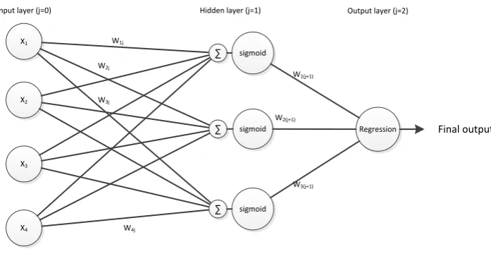
The basic structure of a neural network is that it is an ensemble of neurons connected to levels called layers. This structure is based on the human brain [12]. In this section we will explain the process of the FNN used in this research. In figure 3 is the structure given of the feed forward neural network. The neural network contains three different layers, called the input layer, hidden layer(s) (optional) and the output layer. The neural network is completely connected. Every node in a layer is connected with every node in the next layer, but the nodes are not connected among each other in the same layer. Each connection between two nodes contains a weight wij (i is the node, j is

the layer) [26].

The input layer corresponds with the input variables xi, in our research

these are the weather variables. Each neuron in this layer represents a variable. The neurons from the input layer are connected with the hidden layer and are each affected by a weightwij. The input of a hidden layer is a weighted linear

combination of the output of the neurons from the previous layer[12]. This linear combination is a summation of the inputs, see equation 3[26]. The output of hidden or output layer is a transformation of the weighted linear combination based on a specific transfer/activation function. The most used transfer function is the sigmoid function, see equation 4. In this functionyis the weighted linear combination, see equation 3. The output of the hidden layer is affected by a weight and passes to the input of the next hidden layer or the output layer. The feed forward neural network uses in the output layer a linear regression function as transfer function to create its final output. More information about neural networks can be found in [26].

y=

n

X

i=1

X1

X2

X3

X4

sigmoid

sigmoid

sigmoid

Regression Input layer (j=0) Hidden layer (j=1) Output layer (j=2)

W1j

W4j

W1(j+1)

W2(j+1)

W3(j+1)

Final output

W2j

W3j

∑

∑

∑

Figure 3: Feed forward neural network

S(y) = 1

1 + exp−y (4)

4.2.2 Learning the algorithm

The neural network learns based on a back-propagation algorithm. The basic idea is to adjust the different neuron weights by back-propagating the error between the predicted output and the actual output. In this research adjusting the weights is conducted applying a training function called the Levenberg-Marquardt back-propagation algorithm [31]. This training function minimizes the error to a local minimum.

4.2.3 Hidden neurons and layers

According to Fugon et al. [12] the choice of the number of hidden neurons and layers is important, because a high number of neurons creates complex relations in the model between inputs and outputs and this can lead to overfitting of the data. Trial and error will be applied in this research to obtain the optimal amount of hidden neurons. According to [26] one hidden layer is sufficient for most purposes. Therefore in this research we will use one hidden layer.

5

Related work

been used in previous literature to forecast wind power. Furthermore, we are identifying which forecasting models have been found the most relevant.

The first subsection 5.1 describes which factors have been used by previous literature. The second subsection 5.2 describes which input parameters have been found useful to predict wind power. The final subsection 5.3 describes which forecasting techniques have been used by previous literature to predict wind power.

5.1

Important factors for forecasting wind power

To forecast wind power generated by turbines we have to find out which factors have influence on the forecast of wind power. Based on a literature study we have found three factors which have been found useful to predict wind power. The first factor is the use of different data sources (section 5.1.1), the second factor is the prediction of wind power on different grid areas (section 5.1.2) and the third factor is taking into account the geographical location (section 5.1.3). For each of the factors we describe its importance and relevance for forecasting wind power generated by turbines.

5.1.1 Data sources

Literature has shown that different data sources can be used to predict wind power generated by turbines. Each of these data sources have shown to be useful to predict wind power and therefore we will describe for each data source its use.

Firstly, a large amount of previous research has been done on meteorological data such as HiRLAM and ECMWF [10][36][41][42][44]. Meteorological data is important for day-ahead forecasts since they are covering a horizon of 48 to 72 hours ahead [42]. The data are numerical weather predictions (NWP), measured at 10 meter height which describe the condition of the atmosphere, including important information like wind speed, wind direction, temperature etc. According to Pinson and Kariniotakis [36] and Sideratos and Hatziargyriou [42] NWPs are indispensable for an acceptable performance on short term and long term forecast and their accuracy contributes to the accuracy of wind power predictions.

Secondly, weather stations surrounding the wind turbine or farm [10] have been used as data source to obtain weather data observations. The advantage of using these weather stations is that they provide weather data in a local area near the wind turbine.

Thirdly, the online supervisory control and data acquisition (SCADA) sys-tem has been used to obtain data. The SCADA syssys-tem can provide measure-ments of wind power, wind speed, wind direction and other variables on a real-time basis every minute [42]. The data provided by the SCADA system is measured at the location of the wind turbine or farm and provides the actual operational status. This makes SCADA data valuable since it describes the ac-tual performance of the wind turbine [36]. SCADA data can therefore be used to map the meteorological or weather station data to the state of the turbine and can be used as training data for the prediction model.

measures the weather conditions at different heights using a laser on real-time basis. It can be used to decide placing a turbine in a certain area by measuring the wind profile of that area. An advantage of a LIDAR compared to the SCADA system is that a LIDAR can measure weather conditions on various heights, up to 200 meters, while a SCADA system measures only on the hub height, the height of the turbine rotor.

The combination of different data sources (weather stations and meteoro-logical data) can be mapped to the SCADA data or LIDAR data to create specialized local models for wind power production in specific turbine locations, which might help to improve the prediction of wind power.

5.1.2 Grid area

The prediction of wind power has been applied on different sizes of grid areas. A large amount of research has been focusing on forecasting wind farm pro-duction (e.g. [30], [36], [42]). A wind farm is a group of turbines located in the same area producing wind power. However H. Holttinen and Sillanpaa [14] showed that the aggregation of areas lowers relative share of prediction errors. Their prediction model lowered the prediction error of wind power up to 60%. This result has been obtained when comparing the mean average error (MAE) of 52%-56% from a single turbine with the aggregation of three areas of about 20%. Also Brand et al. [2] and Focken et al. [11] have found that aggregation of wind power improves the quality of the forecast. According to Focken et al. [11] integrating over an extended area, weakly correlated errors underlying predic-tion and measurement cancel out partly due to statistical effects. This results into a reduced prediction error for an area compared to a single turbine.

The size of a aggregation area proposed by H. Holttinen and Sillanpaa [14] is roughly the size of the entire Netherlands. Therefore one aggregation grid area of the Netherlands could decrease the prediction error of wind power. Another grid area which might be applicable is the aggregation on province level.

5.1.3 Geographical location

In many different countries research has been conducted on the prediction of wind power. Because models have been proposed in different countries makes it difficult to evaluate the performance of models [27]. However according to Wang et al. [49], research has been conducted comparing 11 models (which models is unclear), running the same forecasting case. The models were evaluated based on six test cases in Spain, Germany, Denmark and Ireland using the same numerical weather predictions (NWP) as input. Numerical means that each data value is represented as a number.

The results have shown that no forecasting model can perform perfect in any condition, no model was the best in all the cases. Furthermore, the results show that the forecasting accuracy gets worse in complex terrain.

5.2

Input parameters for forecasting models

Forecasting wind power is performed by applying forecasting models. These forecasting models need input data to predict wind power generated by tur-bines. The input parameters which have been found a successful predictor of wind power by literature are taken into account. The input parameters have been selected based on correlation studies reported in literature. This section discusses the input parameters by explaining its importance and relevance.

5.2.1 Wind speed

Wind speed is the most used input parameter to predict wind power generated by turbines. Literature has used average values of wind speed, such as hourly average wind speed [41][10] or monthly average wind speed [30]. To predict wind power for a certain moment in time previous values of wind power and wind speed have been used as input parameters. For example Senjyu et al. [41] have used wind speed predictions on several-hour-ahead, such as data of every six hours interval wind speed has been used for the prediction of six hours ahead and data of one day interval wind speed has been used for the prediction of one day ahead. The number of lagged hours or days required to predict wind power accurately has been determined by performing an autocorrelation and cross-correlation analysis between different variables [10].

A well known formula transforming wind speed into wind power is given in equation 5 [30][41]. The A (m2_{) is the sweep area of the blades. The ρ is}

air density (kg/m3_{) and the V is wind speed (m/s). The air density can be}

calculated as a function of the temperature and pressure.

P =1 2AρV

3 ₍₅₎

In equation 5 one can see that wind power output is proportional to the cube of the wind speed [41]. Therefore a method is required to predict wind speed as accurate as possible, because the error between the predicted and actual wind power value is also proportional to the cube of the error of the predicted and actual wind speed.

Why literature rather use forecasting models to predict wind power rather than wind speed is because of several possible reasons.

Firstly, equation 5 can be applied to forecast wind power for one specific turbine. However the equation has problems to deal with the total wind power output generated from a wind farm. A wind farm is a group of turbines located in the same area producing wind power. It is possible to calculate the wind power generated by one turbine using the predicted wind speed and multiply it by the number of turbines in the wind farm, but this would result in a larger forecasting error because important details have not been taken into account, such as shadowing effects or wake effects caused by other turbines [23]. Wakes are invisible ripples and waves in the atmosphere that can damage turbines and decrease efficiency [22].

Secondly, equation 5 uses a wind speed value measured at one height and therefore does not take into account the wind speed profile, which is the relation between wind speed values on different heights. Wagner et al. [47] state that it is

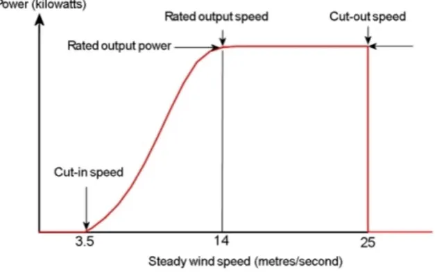
Figure 4: Example of a power curve: turbine power output with steady wind speed1

common to assume that the wind speed profile is continuous based on the wind speed measurements at hub height, which is the height of the turbine rotor. Therefore to predict wind power generated by turbines the wind speed values at hub height are used.

A problem with using the wind speed at hub height is that it ignores the wind speed shear, which is the change of wind speed between two heights. Wagner et al. [47] have found ignoring the wind speed shear could lead to a misinter-pretation of the power performance of the turbine. They have found this result based on measurements using a Laser Imaging Detection and Ranging (LIDAR). A LIDAR can measure the weather conditions at certain heights using a laser. Based on the measurements obtained by the LIDAR they have identified a wind speed profile taking into account the wind speed shear which is different from the wind speed profile ignoring the wind speed shear (only using the wind speed at hub height). This resulted into two different power curves. A power curve shows the relation between the wind speed and the wind power output, see also figure 4 [17][30][44].

The wind speed profiles have been used for deriving an equivalent wind speed, which resulted into a reduction of the scatter in the power curve and therefore into in an improve of the power performance measurement.

5.2.2 Wind direction

the nodes did not all have an adequate level of correlation. Using the irrelevant nodes could result in a poor performance of wind power forecast. Sideratos and Hatziargyriou [42] have found that when the forecast wind direction is between defined limits, NPWs can be considered as relatively accurate. Their reason is because strong winds are difficult to predict but come from known directions due to the topography of the area where the wind farm is located.

5.2.3 Weather stability

Weather stability influences the accuracy of the forecast of among others nu-merical weather prediction (NWP) models. Nunu-merical means that each data value is represented as a number. According to Pinson and Kariniotakis [36] an unstable atmospheric, such as unstable pressure, temperature and/or rel-ative humidity can lead to poor numerical weather predictions and the other way around. To evaluate the global atmospheric situation they have defined a unique representative index for the following Nh hours, called the Meteo-Risk

index (MR-index). The MR-index measures the spread of the weather forecasts at a given time. The most recent forecast is used as a reference and reflects the variability of the older forecast [37]. Low MRI-index indicate there is a stable at-mosphere and high MRI-index indicate there is an unstable atat-mosphere. Pinson and Kariniotakis [37] have calculated the MRI index on a horizon of 24 hours. Since they have used HiRLAM data which provides data every six hours, they have used four sets of wind speed predictions. Plotting the distribution of MRI values against the prediction error they have found that the prediction error increases linearly with the MRI values. Based on this linear relationship they have made the following empirical relation:

e=e0+sMRI (6)

The first part of the right side of equation 6 is the basic part of the error, e0, this is the point where the error line crosses the y-axis, the second part is a

direct consequence of the prediction model sensibility to the weather stability. The sensibilitys is the slope of the linear fitting model. Using this equation a scale factor can be defined for the confidence interval depending on the value of the MRI. The scale factor can be used to enlarge or narrow the interval width for a number of hours Nh. Based on their findings Pinson and Kariniotakis

[37] have defined rules concerning the expected prediction error depending on the MRI values. They have binned the data by MRI values and calculated the cumulative distribution function of the prediction errors for each bin. The results given by this function give the probability with which an error larger than a defined threshold occurs. Based on the defined rules and the results from the distribution function permits one to derive signals that large prediction errors might occur.

5.2.4 Availability

such as mechanical break down or scheduled maintenance. Therefore it is im-portant to plan these factors at moments when wind power prediction is low. This means that the availability of the turbine is very important for the produc-tion of wind power, which is also addressed by Mohandes et al. [33]. Mabel and Fernandez [30] calculate generation hours as follows: generation hour = (total numbers of hours in a month)−(low wind hours + wind turbine maintenance hours + turbine breakdown hours + grid maintenance hours + grid breakdown hours).

For hourly wind power prediction hourly values of availability are required. In case of a single turbine one can correct the predicted wind power output with the availability of the turbine afterwards. But when predicting the total wind power output generated by all the turbines it is important which turbine is active and which one is not. Some turbines produce more wind power than other turbines, because they are larger and have a larger capacity to produce wind power or because wind turbines are located in a wind farm. This means larger turbines have more influence and turbines located in wind farms have less influence on the total produced amount of wind power, because of shadow-ing effects. Therefore it is important to take each turbine its availability into account.

5.2.5 Relative Humidity

Relative humidity of air is dependent on the amount of water vapor in the air, which affects the air density[30]. Mabel and Fernandez [30] and Park et al. [35] have found that relative humidity improves forecasting models to predict wind power. Mabel and Fernandez [30] have found that relative humidity has a dependence on wind power output with a correlation value of 0.4. Furthermore, the monthly variation of relative humidity through the year lays between the 60% and the 90%. Based on these results they have found it important to include relative humidity as one of the input parameters for the prediction of wind power.

5.2.6 Seasonal

Kwon [21] has investigated if there is a seasonal effect in the data. Therefore they have segmented the data in three month sets. The four seasons reveal significant variations of the average error percent. They have found that during the winter the annual production of wind power is relatively high among the four seasons . Furthermore, they have found that the summer exhibits a low wind regime. Also Taylor et al. [44] has found seasonality in their dataset. They have plotted the time against the wind speed and based on this plot one can see that the wind speed is low in the summer months compared to the winter months. Finally, Mohandes et al. [33] have identified a seasonal effect between wind speed and wind power, which they have used for their time series model.

5.2.7 Temperature and pressure

The temperature and pressure have influence on the wind power, since both have influence on the air density. However Kulkarni et al. [19] did not use the feature temperature because the complicated influence of the temperature on wind power would make the selection of a function for a regression model and its fitting difficult. Furthermore, Mabel and Fernandez [30] and Fan et al. [10] have found a low correlation between the temperature and the wind power output and between the pressure and the wind power output. Adding these features did not improve the performance of the models and slowed down the learning process. Therefore these two features have been left out of the models.

5.3

Forecasting models

Forecasting wind power can be performed for different time horizons (e.g. min-utes, hours, days, months). A lot of literature studies have been found in the field of forecasting wind power or wind speed. Literature studies discussing forecasting models for day-ahead (24 to 48 hours) or longer forecast have been analysed. The reason discussing day-ahead forecasting has been explained in the introduction 1. Different types of forecasting models have been identified by literature:

Persistence model: This model is also called Naive predictor model. The wind speed at timet+ ∆twill be the same as it was at timet. [43]

Physical models: These models are using a detailed description of the at-mosphere, topological information and characteristics of the wind tur-bines. The description of the atmosphere are numerical weather predic-tions (NWP) given by a weather service (HiRLAM or ECMWF etc.) and contain information, such as hourly average wind speed, pressure, temper-ature and relative humidity. The topological information contains data about the surroundings of the turbine such as obstacles, roughness and orography. Characteristics of the wind turbine are for instance the height of the rotor of the turbine (hub height) or its location in a wind turbine park. In this research the focus is not on the physical models and there-fore we will not discuss these. However more detailed information can be found in references [24][25][23],

Statistical models: These models such as artificial neural network or regres-sion trees, are based on using a training dataset containing historical mea-surement data. For example to predict wind power, historical measure-ments of weather data is needed such as wind speed, wind direction, etc.

In this research we are going to focus on the prediction of wind power using machine learning techniques. Therefore we are discussing only statistical mod-els. The discussion about physical models and persistence models are beyond the scope of this research.

5.3.1 Statistical models

Many different statistical forecasting models to forecast wind power have been proposed in the literature. To answer the research questions ‘Which forecast-ing models have been proposed in literature?’ and ‘What are the advantages and drawbacks of the proposed models?’ we discuss these proposed statistical forecasting models in detail. Each statistical forecasting model is discussed in a separate subsection and in tables 7, 8 or 9. The subsections and the tables provide the following detailed information: advantages and disadvantages of the model, the used dataset, the input parameters, the output parameter(s) and the country in which the model has been performed.

The statistical forecasting models are discussed in the following order: re-gression trees, time series models, recurrent neural networks (RNN), feed for-ward neural networks, fuzzy-neural networks (FNN) and support vector regres-sion/machine (SVR/SVM).

5.3.1.1 Regression trees

Clifton et al. [7] have performed their research in the USA using the machine learning technique ‘regression trees, see also table 7. They used this technique because it is a technique that can capture non-linear changes. Regression trees are models using a branching structure based on attribute-value pairs to predict an outcome, they are quick to run and easy to update.

Clifton et al. [7] have used the mean value predicted by an ensemble of 100 regression trees to increase the accuracy of the power predictions. Subsets of the training data are used to generate different trees and the predicted power output is calculated by each tree using the same input data. The input data is generated by a turbulence simulator, TurbSIM which creates wind fields. 1796 10 minute wind fields have been created. A wind field consist of a random combination of hub height wind speed between the 3 and 25m/s(height of the turbine rotor), the hub height turbulence intensity (from 5% to 45%) and the wind shear exponent (α) (from−0.5 to 0.5). The wind shear exponent is a value which transforms the wind speed (v0) at the height (h0) to a wind speed (v) at

height (h), see also equation 7. This equation is also called the power law [17]. Besides these three parameters also the operating region has been chosen as input parameter. The output is the prediction of 10 minute mean power values.

v v0

= (h h0

)α (7)

The results show that the ensemble regression tree method predicts two to three times more accurate than the traditional power curve. A power curve is the relation between the wind speed and the output power of a turbine, which is also shown in section 5.2.1.

5.3.1.2 Time series models

time series measurements in the presence of correlations [17]. They have forecast hourly average wind speed up to 48 hours ahead. Table 7 provides information about the dataset, input- and output parameters. Using the power curve they have found the corresponding wind power value. They have found an improving accuracy of 42% compared to the persistence model. More information about the model can be found in reference [17].

Ref. Forecasting model Dataset Input parameters Output pa-rameters

Country

[7] Regression tree 1796 10 Minute Hub height wind speed wind power 10 United States wind field values Turbulence intensity minutes ahead

Wind shear Operating region [17] fractional-ARIMA Four weeks of

wind speed data obtained from four wind gener-ation locgener-ations

Average wind speed (granularity unkown)

Hourly average wind speed val-ues day-ahead (24 hours) and two day-ahead (48 hours)

United States

Table 7: Overview of forecasting models: regression trees and fractional-ARIMA

5.3.1.3 Artificial Neural networks (ANN)

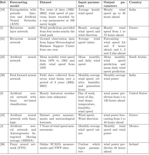
Different types of artificial neural networks (ANN) have been discussed in the literature. Table 8 gives a detailed overview of literature studies which have used ANN to forecast wind speed or wind power. ANN have the ability to learn from experience [8][33], to handle noisy, incomplete or corrupted data[5] and are able to deal with non-linear problems [30]. Furthermore, based on historical data an input-output mapping is constructed [33]. In this section we will discuss the following neural networks: recurrent neural network (RNN), feed forward neural network (FFNN) and fuzzy neural network (FNN).

5.3.1.3.1 Recurrent neural networks (RNN)

Senjyu et al. [41] compared different on-line learning algorithms for training re-current neural networks in Japan (table 8). They have compared a feed forward neural network with a recurrent neural network (RNN). The difference between those two neural networks is that feed forward networks travel one way from the input to the output, whereas recurrent neural networks can travel both direc-tions, meaning they can use their output value as an input value for predicting the next output value. The virtue of recurrent neural networks compared to feed forward networks is that they can establish a dynamic mapping relating input to output sequences [41].

they have found that the RNN performs better than the feed forward neural network.

Barbounis and Theocharis [1] have also forecasted wind power and wind speed values using a recurrent neural network. For more details see table 8. They have found that RNN provide better forecasts compared to the persistent method, the atmospheric and time-series models.

5.3.1.3.2 Feed forward neural network (ANN)

Mohandes et al. [33] have compared a feed forward neural network versus a time series autoregressive model (AR) in Saudi Arabia. The results show that the feed forward neural network outperforms the AR model. Other research conducted by Kulkarni et al. [19] have compared four different statistical techniques: curve fitting, Auto Regressive Integrated Moving Average Model (ARIMA), extrapo-lation with periodic function and feed forward artificial neural network. They have found that wind speed can be predicted based on previous knowledge of wind speed and the local time of the day. Kulkarni et al. [19] have found a periodic behaviour between both parameters by plotting the wind speed of five successive days against the hours of the day. The extrapolation with periodic function and the feed forward neural network performed the best compared to the other two models.

5.3.1.3.3 Fuzzy-neural network (FNN)

Pinson and Kariniotakis [36] have proposed a fuzzy neural network to forecast wind power. This neural network has the ability to adapt and to fine-tune its parameters during on-line operation. Advantages of a FNN compared to the physical models are that it avoids temporal correlations between past and future data, conversion of wind speed from the height of measurement to the hub height of wind turbines, spatial projection of the meteorological wind speed forecast from the NWP to the level of the wind farm and correction of the wind park output for factors affecting the total production [36].

5.3.1.4 Support vector regression/machine

Ref. Forecasting model

Dataset Input

parame-ters

Output pa-rameters

Country

[19] Extrapolation with periodic func-tion and Artificial Neural Networks (ANN)

Ten years of data (1992-2002) wind speed of pre-vious hours recorded by a cup anemometer at 100 meter height

Average hourly wind speed

Hourly wind speed up to 48 hours ahead

India

[1] Recurrent multi-layer network

Wind predictions provided from four nodes nearby the wind park

Hourly average wind speed and wind direction

Hourly wind speed from 1 to 72 hours ahead

Greece

[41] Recurrent neural network

Ground observation data from Japan Meteorological Business Support Center from one year

Average wind speed values

Forecasting wind speed 3,6 and 9 hours ahead, and 1, 2 and 3 day-ahead

Japan

[33] Artificial neural network

Mean monthly wind speed from 1970 to 1982 and daily wind speed from 1970

Mean monthly and daily wind speed

Mean monthly wind speed prediction and mean daily wind speed prediction

Saudi Arabia

[30] Feed forward neural network

Field data collected from seven wind farms over a period of 3 years (2002-2005)

Monthly average wind speed, rel-ative humidity and generation hours Monthly average wind power India

[8] Artificial neu-ral network with fuzzy set-based classification

Hourly historical weather data (size unknown)

Day of week, hour of day, load shape, temperature, humidity, wind speed

wind power pre-diction from 1 to 120 hours ahead

United States

[42] Artificial neural network with fuzzy logic

Dataset power measure-ments and meteorological forecasts

Wind speed, Wind direction

wind power fore-casting from 1 to 48 hours ahead

Greece

[4] Artificial neu-ral network and Autoregressive In-tegrated Moving average (ARIMA)

7 Years of wind speed mea-surements

Monthly average wind speed val-ues

Monthly wind speed and wind power

Mexico

[36] Fuzzy neural net-work (FNN)

Online SCADA measure-ments and NWP data

Unclear which input parame-ters

wind power pre-diction 48 hours ahead

Ireland

Table 8: Overview of forecasting models with its input and output features

5.3.1.5 Discussion

Ref. Forecasting model

Dataset Input

parame-ters

Output pa-rameters

Country

[10] Bayesian clustering with Support vector regression

10 minutes data from the wind farm, obser-vations from a meteoro-logical tower, hourly ob-servations from surround-ing weather stations and hourly meteorological fore-cast at the wind farm its location Wind speed, wind direction, humidity Hourly wind power genera-tion from 1 to 48 hour ahead

United States

[32] Support vector ma-chine vs. Multilayer perceptron

Daily wind speed data of 12 years between 1970 and 1982

Mean daily wind speed data

Mean daily wind speed data

Saudi Arabia

Table 9: Overview of forecasting models with its input and output features

forecast of wind power generated by turbines. It is hard to compare forecasting techniques and determine which one works best, because the previous research have analysed different techniques on different datasets in different countries.

Therefore in our research we compare two forecasting models, feed forward neural network and a random forest which have been explained in section 4. Based on our analysis on the forecasting models we have found that differ-ent types of neural networks are good predictors on long term forecasting and according to Mohandes et al. [33] and Barbounis and Theocharis [1] neural net-works perform better than time series. Furthermore, Barbounis and Theocharis [1] have found that Recurrent Neural Networks performs better than the Feed forward neural network.

The main advantages using neural networks are because neural networks have the ability to learn from experience, to handle noisy and incomplete data. Furthermore, maybe one of the most important advantages is neural networks can handle linear problems, because the prediction of wind power is a non-linear problem. A drawback of neural networks is that they have a high com-putational complexity.

Other forecasting models such as SVM or Recurrent neural network have not been taken into account to use as a forecasting models in this research. The main reason is because lack of time.

5.4

Feature selection methods

To identify the right input parameters different selection methods have been applied in the literature. Fan et al. [10] have selected their features using the correlation function shown in equation 8. In this equation the Cov(g, s) is the covariance of generation g and wind speeds and σg and σs are the