Technical Term Extraction Using Measures of Neology
Christopher Norman
Royal Institute of Technology
The University of Tokyo
[email protected]
Akiko Aizawa
National Institute of Informatics
The University of Tokyo
[email protected]
Abstract
This study aims to show that frequency of occurrence over time for technical terms and keyphrases differs from general lan-guage terms in the sense that technical terms and keyphrases show a strong ten-dency to be recent coinage, and that this difference can be exploited for the auto-matic identification and extraction of tech-nical terms and keyphrases. To this end, we propose two features extracted from temporally labelled datasets designed to capture surface leveln-gram neology. Our analysis shows that these features, cal-culated over consecutive bigrams, are highly indicative of technical terms and keyphrases, which suggests that both tech-nical terms and keyphrases are strongly bi-ased to be surface level neologisms. Fi-nally, we evaluate the proposed features on a gold-standard dataset for technical term extraction and show that the proposed fea-tures are comparable or superior to a num-ber of features commonly used for techni-cal term extraction.
1 Introduction
Keyphrases are terms assigned to documents, con-ventionally by its authors, that are intended chiefly as an aid in searching large collections of docu-ments, as well as to give a brief overview of the document’s contents. Technical terms are words or phrases that hold a specific meaning in spe-cific domains or communities. Keyphrases are closely related to technical terms in the sense that the keyphrases assigned to a document are gen-erally selected from the terminology of the doc-ument’s domain. Keyphrases and technical terms show considerable conceptual overlap, and by tension, so do keyphrase and technical term ex-traction. As a consequence, these two are closely
related research topics. In this study we will see technical term extraction and keyphrase extraction as distinct but related. We will take the view that the technical terms in a scientific article are likely candidates to be keyphrases for the document and consequently that technical term extraction meth-ods might also be useful in keyphrase extraction.
We will show that features that capture the neol-ogy of term candidates can be used to extract tech-nical terms, and that the basic assumptions that en-able this extraction also hold true for keyphrases.
This paper is organized as follows: We first dis-cuss how technical terms and keyphrases differ from general language terms in terms of neology. We then define features that capture this differ-ence and analyze these features statistically using the SemEval-2010 dataset (Kim et al., 2010) and a gold-standard for technical term extraction derived from the same dataset (Chaimongkol and Aizawa, 2013). Our analysis shows that the proposed fea-tures reliably separate positive from negative ex-amples, both of technical terms and of keyphrases. Furthermore, the histograms for the proposed fea-tures are very similar when calculated for cal terms and keyphrases, suggesting that techni-cal terms and keyphrases have very similar neo-logical properties. Finally, we demonstrate that this statistical bias can be used to reliably extract technical terms in a gold-standard dataset, and that the proposed features are comparable or superior to other features used in technical term extraction, with an F-score of 0.509 as compared to 0.593, 0.367, 0.361, and 0.204 for affix patterns, tf-idf, word shape, and POS tags respectively.
2 Related works
Most technical term extraction systems work fairly similarly to keyphrase extraction systems, using an initial n-gram or POS tag-based filtering to identify term candidates, then proceeding to nar-row this list down using machine learning algo-rithms on various kinds of document statistics such as term frequency or the DICE coefficient (Justeson and Katz, 1995; Frantzi et al., 2000; Pin-nis et al., 2012). For an in-depth summary of the state-of-the-art in technical term extraction, we re-fer to Vivaldi and Rodr´ıguez (2007). For a sum-mary of the state-of-the-art in keyphrase extrac-tion, which largely follow the same pattern, we re-fer to Hasan and Ng (2014). The main difre-ference in implementation might simply come down to a choice in top-level machine learning approach: in technical term extraction it makes sense to view the problem as a binary classification problem, whereas in keyphrase extraction it makes more sense to see the problem as a ranking problem.
Approaches based on frequency statistics ex-tracted from the documents themselves are, how-ever, not without their drawbacks. To begin with, for document statistics to be meaningful we will need a dataset that is large enough, consisting of documents that are large enough individually. We might also encounter problems if the documents are too large, because then the statistics might be drowned out by noise in the data (Hasan and Ng, 2014). We should also be careful about the topi-cal composition of the data set – if the dataset only contains documents from a single domain, then we will have to approach the problem very differently than if the dataset contains documents from mul-tiple domains. Preferably, we want methods that do not make these kinds of assumptions about the data set, methods that can be applied to documents of any size, and to document collections of any size or of any topical composition. In the best of worlds, we want methods that can be applied to document collections consisting of a single docu-ment, or even a single sentence.
One way to go beyond simple document statis-tics is to use external, pregenerated resources. To give some examples of this, Medelyan and Wit-ten (2006) use a pregenerated domain thesaurus to conflate equivalent terms and to select candidates that are thematically related to each other, Hulth et al. (2006) use a pregenerated domain ontology to select candidates whose synonyms, hypernyms,
and hyponyms also appear in the text, and Lopez and Romary (2010) use a terminology database as one way to measure the salience of term candi-dates for keyphrase extraction in scientific articles. Medelyan et al. (2009) use a somewhat more in-direct external resource by taking the frequency by which a term candidate appears in Wikipedia links, divided by the frequency by which it ap-pears in Wikipedia documents. The idea behind using external resources is that human annotators generally perform better than automatic systems, and resources produced by human beings are thus much more reliable than automatic methods, even if the resources themselves are only obliquely re-lated to keyphrases.
However, depending on the speed by which the terminology of the subject field changes, any previously generated resource might become out-dated very quickly. In a subject field such as law, where the terminology only changes impercepti-bly over time (Lemmens, 2011), this is unlikely to be an issue, but in a quickly changing subject field such as information science, where the terminol-ogy has been reported to change by as much as 4% per year (Harris, 1979), it is likely that pregener-ated resources will lag behind recent terminolog-ical developments. One selling point of the auto-matic extraction of keyphrases or technical terms is that automatic methods are able to respond to changes in the terminology of a subject field with the same speed that the terminology changes, but if we rely on pregenerated resources then we for-sake this advantage, since these are unlikely to in-clude terminology that only recently appeared in the subject field.
3 Theoretical basis
would allow us to obtain more recent data than the Google Ngrams dataset, which only contains frequencies of occurrence from before 2008.
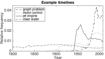
Figure 1: Example timelines (frequency of oc-currence) for three technical terms and one non-technical term. The frequencies of occurrence for each timeline has been normalized to sum to one to fit all graphs in the same diagram.
In order to develop some intuition about how technical terms are adopted, let us look at the timelines for some technical terms in the Google Ngrams dataset (Figure 1). To begin with, all the technical terms (graph problem,motor control, and jet engine) are relatively recent coinage, and none of them were in use in the 19th century. In all three cases, there is some point in time at which the term gained momentum and began to surge in frequency. This characteristic is fairly typical of technical terms, although we can of course find general language terms that exhibit the same pat-tern of adoption. By contrast, the non-technical term (clear water) has been in use throughout the 19th and 20th century. Unlike technical terms, general language do not have generally observable characteristics, and the shape of the timelines vary greatly from case to case. The defining character-istic instead seems to be one of contrast: general language terms seldom have the steep curves that we can observe of the technical terms here.
We will formalize this difference and examine it statistically in the later parts of this study.
Of course, our ability to find neologisms by ex-amining the frequency of occurrence of their sur-face forms necessitates that technical terms gener-ally do not share surface forms with general lan-guage terms. If such is the case, then the general language senses of the terms are likely to drown out the technical term senses. For instance, con-sider a term likewormin computer security. The vast majority of the occurrences of the unigram
worm in the Google Ngrams dataset are likely to be of the biological variety, and it is consequently impossible to tell from the Google Ngrams dataset alone that the computer security term only ap-peared in the later half of the 20th century1. For-tunately, the case where technical terms coincide with general language terms is rare, at least when considering terms composed of multiple words.
The overall recency of coinage of technical terms depends on the subject field – the major-ity of the terminology in e.g. computer science consists of terms whose surface forms were in-troduced no earlier than the middle of the 20th century, whereas subject fields such as mathemat-ics and physmathemat-ics include terminology coined in the 19th century or earlier. Consequently, if we plot the frequency of usage of a neologism over time we would expect to see a curve similar to those in Figure 1, but we should expect that the curves may be shifted to the left or to the right, largely depending on the subject field.
Why are technical terms so often neologisms? It turns out that general language, which is what is ordinarily studied in linguistics, and special lan-guage, which is what we actually encounter in the documents commonly used for keyphrase extrac-tion, differ quite substantially in linguistic aspects (Sager et al., 1980). One difference is that sur-face level neologisms are seldom created in gen-eral language. Rather, the creation of new sur-face forms generally occur in special language, from which the term might later be transferred to general language (Sager et al., 1980, p. 287). Consequently, terms that have appeared recently, given some specific point in time, are likely to be domain-specific at that point. The longer that has passed since the adoption of the term, the more likely it is that the term has been adopted into gen-eral language.
4 Measures of neology
We have noted that the shape of the timelines seem to indicate whether a given term is recent coinage, but in order to use these as input to machine learn-ing algorithms, we need to distill the high dimen-sional data into low-dimendimen-sional features that re-tain the neological information.
1However, the termcomputer wormis a surface level
ne-ology. We might thus observe that new senses of the unigram
What we want to extract is of course not neces-sarily the shape of the timelines, but whether the occurrences of then-grams predominantly occur in the far right side on the time axis. In other words, we want to determine if the timeline is mainly concentrated on the right side. This is sim-ple to do using statistical measures such as the mean and the standard deviation of the curves.
Letfi
y denote the frequency of ann-grami in yeary. Thenpi(y) = f
i y
Σyfyi constitutes a probabil-ity densprobabil-ity function, with the expected value:
µi=
X
y pi(y)·y=
P
yfyi·y
P
yfyi
How this ”mean” should be interpreted might not be completely intuitively obvious, but for our purposes here it is enough to note that µi indi-cates where the curve is mainly concentrated. If the curve is concentrated around higher values of ythen we have, by definition, a surface level neol-ogism.
We can take the standard deviation ofpiin the same way:
σ2 i =
X
y pi(y)·(y−µi) 2=
P
yfyi·(y−µi)2
P
yfyi
The standard deviation σi then yields a mea-sure of how much the probability density is con-centrated aroundµi, in other words, how ”steep” the probability density is. A low standard devia-tion consequently indicates that the term has been adopted or abandoned rapidly. Low standard de-viation should thus in general imply either surface level neologisms or fads. If we are only interested in how quickly a term has been adopted and not how quickly it might have been abandoned, then we can take a one-sided ”standard deviation”, by separating out they for which y < µi, but this does not seem to make much difference for the sake of the separability of technical terms. Those terms that have been adopted quickly also appear to be likely to quickly fall into relative disuse.
We should hasten to point out that there does not seem to exist any theoretical reasons to use the mean and standard deviation in this way. For in-stance, using the peak of the curve (i.e. the mode of the distribution) might have more intuitive ap-peal, since this should correspond to the point in time at which the term was in its most widespread use. However, the Google Ngrams dataset is
of-ten plagued by severe noise, in particular for less commonly usedn-grams such as technical terms, and the peaks of the timelines are thus likely to be spurious. The mean and the standard deviation may be crude measures of shape, but they have the advantage of being robust against noise, and can generally be used with good results even for very noisy timelines.
Other intuitively appealing features, such as the first order derivatives of the timelines or the skew-ness of pi have turned out not to be very useful, presumably because of the noise.
5 Statistical properties of technical terms
and keyphrases
In this section, we examine statistically the fea-tures we propose, and show that both technical terms and keyphrases are strongly biased towards certain values for our features. We also under-line the relationship between technical terms and keyphrases by showing that these are very similar in terms of neology.
To analyze keyphrases we will use the SemEval-2010 dataset (Kim et al., 2010), one of the most commonly used gold standards for keyphrase extraction. To analyze technical terms we will use a dataset consisting of the abstracts from the SemEval-2010 dataset manually anno-tated by two annotators such that all the technical term spans have been labeled (Chaimongkol and Aizawa, 2013). Since this dataset was constructed from the abstracts of the SemEval-2010 dataset we assume that these datasets are similar enough that analyzing and comparing the statistical properties of these two datasets is meaningful.
For the analysis in the following section, we construct three classes of data:
• We extract the n-grams that are part of the spans labeled as technical terms in the Chaimongkol-Aizawa dataset to obtain one set of positive examples of technical terms.
• We extract the constituentn-grams from the gold-standard keyphrases from the SemEval-2010 training dataset (using the combined set) to obtain one set of positive examples of keyphrases
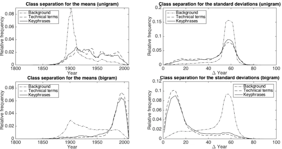
Figure 2: Class separation between technical terms, keyphrases, and background terms overµi(left) and σi(right), when considering unigrams (top), and bigrams (bottom). Histogram bin size was set to 2 in all cases. The resulting histograms have been smoothed using Matlab’s default settings (moving average with span 5) and normalized to sum to one.
set of negative examples of both technical terms and keyphrases.
We could of course extract negative examples of keyphrases from the SemEval-2010 dataset, but it is not so clear that these would all unquestionably be negative examples of keyphrases. Given that inter-annotator agreement is generally very low for keyphrases, this set might well contain terms that could reasonably be considered keyphrases by other annotators. We here assume that the negative examples of technical terms also consti-tute negative examples of keyphrases, and that this set is less likely to contain borderline cases of keyphrases. Only using three classes of data also simplifies both the exposition and the processing.
For these three classes of n-grams, we ex-tract the corresponding timelines from the Google Ngrams dataset over the period 1800–2008, and we calculate the meansµand standard deviations σfrom these as defined in the preceding section. To analyze the featuresµ and σwe plot the his-tograms of the values for the technical term n-grams and the keyphrasen-grams versus the back-groundn-grams (Figure 2).
In order for the features to be useful for either technical term extraction or keyphrase extraction
we would like to see as little overlap as possi-ble between the histograms of the positive and the negative examples. This seems to hold true for the bigrams, but not for the unigrams. In the unigram case we can see only a weak tendential difference in the histogram densities of the positive and neg-ative examples.
We should point out that the mode of the his-togram densities for the negative examples fall very close to the mean and standard deviation of a uniform distribution over the period 1800–2008. These would occur around 1904 and 60.48 respec-tively.
In all cases, the histograms for the technical terms and the keyphrases are very similar. This might not seem very surprising given that all the data is derived from the SemEval-2010 dataset, but it bears mentioning that these were annotated by different people, and more importantly, using very different annotation criteria.
We omit trigrams and higher order n-grams from consideration.
n-grams, such as technical terms, as well as higher ordern-grams are likely to be missing (see Table 1). This problem is not very severe for unigrams and bigrams, but technical term trigrams suffer from data sparsity problem severe enough to es-sentially render them useless. Part of this problem might be due to the large mismatch between the dataset used for evaluation, and the Google Ngram dataset used to identify neology. If we were to use an external dataset from a more similar domain to the evaluation set, then we would expect to find a greater portion of the n-grams in the external dataset.
Technical terms Background
Unigram 97.5 % 100 %
Bigram 85.0 % 97.0 %
Trigram 25.5 % 71.0 %
Table 1: The ratio of n-gram in each class in the Chaimongkol-Aizawa dataset that occur in the Google Ngrams dataset. The percentages have been generated by chosing a random sample of 200 unigrams of each class, 200 bigrams of each et c., and checking if the n-gram occur in the Google Ngrams dataset using the web interface.
6 Evaluation on technical term
extraction
In order to demonstrate that neology, as character-ized by the featuresµandσ, can be used to auto-matically extract technical terms, we implement a simple technical term extractor using these as fea-tures. We generally follow the approach taken by Chaimongkol and Aizawa (2013) and implement a conditional random field model to BIO-tag the dataset. The major difference in implementation is that we use the neology features extracted from Google Ngrams in the term extractor, and that we do not use features based on clustering.
For the sake of our CRF model, bigrams and unigrams are sufficient, since what we want to do is to obtain features corresponding to each node (i.e. to each unigram) and features correspond-ing to the links between the nodes (i.e. to each bigram). We might in theory achieve better per-formance with higher ordern-grams, but in real-ity the results would be severely hampered by the sparsity problems for higher ordern-grams.
Similarly to Chaimongkol and Aizawa, we im-plement a CRF model using the freely available
state-of-the-art CRF framework CRFSuite2, using five different feature sets:
1. POSTAGSusing the Stanford POS tagger3.
2. WORD SHAPEfeatures extracted similarly to Chaimongkol and Aizawa. These include bi-nary features such as whether the current to-ken is capitalized, uppercased, or alphanu-meric.
3. AFFIXES of length up to 4 characters ex-tracted for all tokens. In other words, for the tokencarbonizationwe would extractcarb-, car-,ca-,c-,-tion,-ion,-on, and-n.
4. TF-IDFfor each unigram and bigram in the dataset.
5. NEOLOGYbased features, in other words the mean and standard deviation of the Google Ngrams timeline as described in section 4.
The mutual information between each neigh-boring token in the dataset has also been tried, but this turned out to not have any perceptible effect on the results.
Because CRFSuite cannot handle continuous features, such as tf-idf, µ, or σ, we had to resort to discretizing these by binning. Appropriate bin sizes were established experimentally.
We apply the system on the labeled dataset where we attempt to binary classify each token into positive and negative examples, where posi-tive examples are those that are part of a technical term compound, and negative those that are part of the background. We use the full dataset, and evaluate using 10-fold cross-validation.
Using all features, the system achieves an F-score around0.7for the technical term tokens, and an F-score around0.9for the non-technical term tokens.
To compare the different features with each other, we evaluate their performance individually (Table 2). The best performing feature turns out to be the affixes, although our neology features are quite comparable in performance. Neology per-forms better than all other features except affixes.
2http://www.chokkan.org/software/
crfsuite/
3http://nlp.stanford.edu/software/
Technical terms Non-technical terms
P R F1 P R F1
[image:7.595.167.431.64.154.2]POS tags 0.734 0.118 0.204 0.835 0.991 0.906 Word shape 0.659 0.248 0.361 0.853 0.971 0.909 Affixes 0.673 0.530 0.593 0.900 0.943 0.921 tf-idf 0.600 0.244 0.367 0.852 0.964 0.904 Neology 0.637 0.423 0.509 0.881 0.947 0.913
Table 2: Term extractor performance in terms of correctly labeled tokens. Here, the system is only using a single feature class in each trial in order to compare the relative performance of each feature class.
Technical terms Non-technical terms
P R F1 P R F1
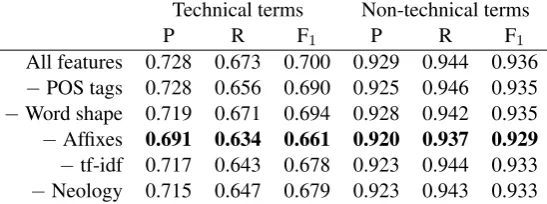
All features 0.728 0.673 0.700 0.929 0.944 0.936 −POS tags 0.728 0.656 0.690 0.925 0.946 0.935 −Word shape 0.719 0.671 0.694 0.928 0.942 0.935 −Affixes 0.691 0.634 0.661 0.920 0.937 0.929
−tf-idf 0.717 0.643 0.678 0.923 0.944 0.933 −Neology 0.715 0.647 0.679 0.923 0.943 0.933
Table 3: Term extractor performance in terms of correctly labeled tokens. Here, the system is using all but one feature class in each trial in order to compare the relative performance drop when each feature class is removed from the classifier.
It might be mentioned that these results are calcu-lated over all tokens, even those where the neol-ogy features are missing because the correspond-ingn-grams do not occur in the Google Ngrams dataset. It is likely that the performance of the ne-ology features would be higher if these were ex-cluded from consideration. This might seem like cheating, but we should consider what would hap-pen if we were to use another dataset with greater coverage, or some future improved version of the Google Ngrams dataset with greater coverage.
We also perform an ablation experiment to see how much the performance drops when exclud-ing individual feature classes (Table 3). Similarly, the biggest drop occurs when excluding affixes. In this case, however, the differences between the different features are quite modest, which seems to imply that each single feature does not contain much information that is not also contained in the other features.
Compared to tf-idf, the neology feature is of-ten able to correctly identify technical term spans containing terms which are also frequent in the remainder of the document collection, such as technical terms containing words like: network, computer, function, algorithm, complexity, data, server,model, orvector. It is much less easy to summarize where neology works well compared
to the other features besides tf-idf.
Neology features are much less effective when the technical terms coincide with general language terms, for instanceworm,precision, orMAP. This is generally only a problem in the unigram case, and bigrams such as computer worm or average precisiongenerally do not have this problem.
7 Discussion
In this paper we have shown that technical terms tend to be recently coined, and that this statistical tendency is strong enough that it allows us to ex-tract technical terms with reasonable accuracy. We have also shown that this statistical feature of tech-nical terms also seem to hold true for keyphrases, and we therefore maintain that it is reasonable that similar features might also be useful in keyphrase extraction. We should not expect equally high per-formance in keyphrase extraction, however, since in keyphrase extraction we are not only interested in whether the output keyphrases are terms in the relevant domain, but also that they are significant in the document under consideration. What we do suggest is that neology can be useful for keyphrase extraction when used in concert with other fea-tures such as tf-idf that indicate significance or topicality.
[image:7.595.163.437.199.301.2]keyphrases fundamentally depends upon the as-sumption that these are biased in certain ways. For instance, a common assumption taken in keyphrase extraction is that keyphrases are biased to occur more frequently at certain positions in the document. Another common assumption is that technical terms and keyphrases are biased to occur with different frequencies in certain communities, or that the contexts in which keyphrases and tech-nical terms appear differ between different com-munities. Similarly to the position and community bias of keyphrases, we suggest that keyphrases also have a time bias, that the keyphrases of a document are skewed to be overrepresented in the contemporary and subsequent literature, but likely to be absent or severely underrepresented in the precedent literature.
The very high values of the means, and the very low values of the standard deviations ob-served for the technical terms in section 5 sug-gests that the majority of the technical term bi-grams studied in this paper come from terms that only appeared after 1950. This might be explained by the fact that the datasets we use here are de-rived from the SemEval-2010 dataset, which is strongly biased towards computer science litera-ture. It seems reasonable that the separation be-tween the classes should generally be stronger in subject fields where the terminology tends to be very recent coinage than in fields with more ma-ture terminology. If this is true, then the ap-proach we propose here should work well for sub-ject fields where the terminology is rapidly chang-ing, and where the need for automatic extraction methods is arguably the greatest.
Acknowledgements
This work was supported by the Grant-in-Aid for Scientific Research (B) (15H02754) of the Japan Society for the Promotion of Science (JSPS).
References
Panot Chaimongkol and Akiko Aizawa. 2013. Uti-lizing LDA Clustering for Technical Term Extrac-tion.Proceedings of the Nineteenth Annual Meeting of the Association for Natural Language Processing, Nagoya, pages 686–689.
Katerina Frantzi, Sophia Ananiadou, and Hideki Mima. 2000. Automatic recognition of multi-word
terms: The C-value/NC-value method.
Interna-tional Journal on Digital Libraries, 3:115–130.
Jessica Harris. 1979. Terminology change: Effect on index vocabularies.Information Processing & Man-agement, 15(2):77–88.
Kazi S. Hasan and Vincent Ng. 2014. Automatic Keyphrase Extraction : A Survey of the State of the Art.Acl, pages 1262–1273.
Anette Hulth, Jussi Karlgren, and Anna Jonsson. 2006. Automatic keyword extraction using domain
knowl-edge. Computational Linguistics and Intelligent
Text Processing, pages 472–482.
John S. Justeson and Slava M. Katz. 1995. Technical terminology: some linguistic properties and an al-gorithm for identification in text.Natural Language Engineering, 1:9–27.
Su Nam Kim, Olena Medelyan, Min-Yen Kan, and Timothy Baldwin. 2010. Semeval-2010 task 5: Au-tomatic keyphrase extraction from scientific articles.
Proceedings of the 5th International Workshop on Semantic Evaluation, pages 21–26.
Koen Lemmens. 2011. The slow dynamics of legal language: Festina lente? Terminology, 17:74–93. Yuri Lin, Jean-baptiste Michel, Erez L. Aiden, Jon
Orwant, Will Brockman, and Slav Petrov. 2012. Syntactic Annotations for the Google Books Ngram Corpus.Proc. of the Annual Meeting of the Associa-tion for ComputaAssocia-tional Linguistics, pages 169–174. Patrice Lopez and Laurent Romary. 2010. HUMB : Automatic Key Term Extraction from Scientific
Ar-ticles in GROBID. Proceedings of the 5th
Inter-national Workshop on Semantic Evaluation, pages 248–251.
Olena. Medelyan and Ian H. Witten. 2006. Thesaurus
based automatic keyphrase indexing. Proceedings
of the 6th ACM/IEEE-CS joint conference on Digital libraries, pages 6–7.
Olena Medelyan, Eibe Frank, and Ian H. Witten. 2009. Human-competitive tagging using automatic keyphrase extraction.Proceedings of the 2009 Con-ference on Empirical Methods in Natural Language Processing, 3:1318–1327.
M¯arcis Pinnis, Nikola Ljubeˇsi´c, Dan S¸tef˘anescu, In-guna Skadin¸a, Marko Tadi´c, and Tatiana Gornos-tay. 2012. Term Extraction, Tagging, and
Map-ping Tools for Under-Resourced Languages.
Pro-ceedings of the 10th Conference on Terminology and Knowledge Engineering, pages 193–208.
Juan C. Sager, David Dungworth, and Peter F.
McDon-ald. 1980. English special languages: principles
and practice in science and technology. John Ben-jamins Publishing Company.