Improving the Morphological Analysis of Classical Sanskrit
Oliver Hellwig
Düsseldorf University, SFB 991
ohellwig@
phil-fak.uni-duesseldorf.de
Abstract
The paper describes a new tagset for the morphological disambiguation of Sanskrit, and compares the accuracy of two machine learning methods (CRF, deep recurrent neural networks) for this task, with a special focus on how to model the lexicographic information. It reports a significant improvement over previously published results.
1 Challenges of Sanskrit Linguistics and Related Research
Classical Sanskrit is a strongly inflecting Old Indo-Aryan language that developed out of earlier Vedic dialects in the middle of the first millenium BCE. Ever since, Sanskrit has been the main medium for transmitting the large corpus of religious, philosophical, scientific, and literary texts that shaped the intellectual history of ancient India.
Sanskrit poses considerable challenges for NLP at the levels of tokenization, lemmatization, and mor-phological analysis (Kulkarni and Shukla, 2009). These three steps are deeply intertwined in Sanskrit, because single word forms (padas) are merged by a set of phonetic rules called Sandhi “connection” into larger strings. In order to analyze a sentence at the morphological and lexical level, an NLP tool must be able to simultaneously resolve the Sandhis, and to detect the correct morphological and lexical path in the resulting lattice of word hypotheses. As a consequence, the tokenization of a sentence is guided by its lexical and morphological analyses. Due to these linguistic peculiarities, morphological ambiguity is introduced on three levels:
Inherent : Isolated Sanskrit forms are frequently ambiguous. The verbal formgacchati, for example, has three readings as 3rdSG.PRof the verbgam‘to go’ (“(s)he / it goes”), L.SG.M. of the present participle of this verb (“in the going [some referent]”), and L.SG.N. of the same participle.
Sandhi : When morphologically unambiguous forms such as draupad¯ı(N.SG.F. of draupad¯ı‘name of a woman’) are processed with Sandhi rules, they can become ambiguous. While the sentence
draupad¯ı gacchati ‘Draupad¯ı goes’ allows only one reading of draupad¯ı, the sentence draupad¯ı ¯agacchati ‘Draupad¯ı arrives’ is further processed by the Sandhi rule ¯ı + ¯a = y¯a, resulting in
draupady¯agacchati. When this string is analyzed with an NLP tool, the sequence-y¯a- can be re-solved into (1) the “correct” source phonemes¯ı + ¯a, but also into (2)i + ¯a, (3)ya + a, (4)ya + ¯a, (5)
y¯a + a, or (6)y¯a + ¯a, where solutions (1), (2), (5), and (6) represent lexico-morphologically, but not necessarily semantically valid readings.1 The morphological analyzer (MA) has to decide between
three readingsdraupad¯ı(N.SG.),draupadi(V.SG.), anddraupady¯a(I.SG.), which are distinct in their un-Sandhied, phonetically disambiguated forms.
bahuvr¯ıhicompounds : Sanskrit has a highly productive class of compounds calledbahuvr¯ıhis (“much rice”), which form possessive expressions. Compounds of this class behave like adjectives, because they inherit the inflectional information from their governing possessors. While the non-possessive This work is licensed under a Creative Commons Attribution 4.0 International Licence. Licence details: http: //creativecommons.org/licenses/by/4.0/.
1(2) “O Draupad¯ı, he/she/it comes”; (5*) “With Draupad¯ı ... in the not-going”; (6) “He/she/it arrives together with Draupad¯ı”
compound bahu-annam ‘much food’ is inflected according to the grammatical class of its final memberanna ‘food’ (neutre noun on short a), it takes over the inflectional class of the govern-ing termstr¯ı ‘woman’, when used in thebahuvr¯ıhiconstruction bahu-ann¯a2 str¯ı ‘a woman who
has much food’. Morphological ambiguity is introduced in constructions such as mah¯a-vr.ks.am
udy¯anam‘big-tree + garden’, where the first elementmah¯a-vr.ks.amhas two readings:
1. possessive compound: “the garden that has (a) large tree(s)”.mah¯a-vr.ks.amis N. or A.SG. fol-lowing the selected morphological information of udy¯anam(N. or A.SG.N.), and its gender changes from M. to N.
2. non-possessive compound: “the big tree [and] the garden”.mah¯a-vr.ks.amshould preferably be analyzed as A.SG.M.
As in the case of Sandhi, resolving such cases correctly requires long-range contextual information. Tagging Sanskrit texts requires a robust algorithm. Apart from the morphological disambiguities just described, the algorithm should be able to handle texts from a wide spectrum of domains, and from a timespan of over 2,500 years. Classical Sanskrit is generally assumed to be regulated by P¯an.ini’s grammar As.t.¯adhy¯ay¯ı (Scharfe, 1977) on the phonetic, morphological, and – to a certain degree – the syntactic level, and by the large dictionaries such as the Amarako´sa (approx. 3.-5. c. CE) and the Abhidh¯anacint¯aman.i (12. c. CE; see Katre (1991)) on the lexicographic level. However, the actual use in texts may frequently diverge from such an ideal language.3
Although better explored than Middle Indo-Aryan languages (see, for instance, Alfter and Knauth (2015)), Sanskrit is still a low-resource language from the perspective of NLP. Research on morpho-logical disambiguation concentrates on building analyzers with a high coverage of valid word forms (Huet, 2005; Jha et al., 2009a; Mishra, 2009). Frameworks for analyzing complete sentences either rely on Finite State methods (Huet, 2006), or a combination of rule-based and statistical methods (Hellwig, 2015).
The present paper adopts a two-stage approach that resembles the methods proposed in Hajiˇc and Hladká (1998). During the first stage, Sandhis are resolved, and the most probable lexical reading is detected using a factorized bigram language model. Morphological disambiguation, the topic of this paper, is performed during the second stage. At this point, the algorithm has access to the most probable lexical analysis of each word, and to the corresponding morphological reading(s) that are determined using a rule-based morphological analyzer. The experiments reported below deal with the question of how morphological ambiguities can be resolved in this second stage. It is important to keep in mind that the lexical and morphological information can contain errors, if the algorithm does not select the correct lexical reading in the first stage.
2 Method
2.1 Tag set
The inflectional morphology of a Sanskrit word can be described by five, partly incompatible categories. Nouns, adjectives, pronouns, and verbal participles are inflected by (1) eight cases, (2) three numbers (SG., DU., PL.), and (3) three genders (M., F., N.). Unmarked forms of these word classes are used in compound formation. Finite verbal forms are marked for number and (4) person (1st, 2nd, 3rd), and (5) by a complex system of tenses and modes. The rule based morphological analyzer produces fine-grained annotations that cover these five morphological categories. Because the classification methods used in this paper require a single output variable from a nominal scale, an obvious approach would use the Cartesian product of the five morphological categories as target variable. However, this approach unnecessarily complicates the learning process, because most feature combinations cannot cooccur in the morphological analysis of a single word. As a consequence, Hellwig (2015) reduced the tag set used
2-¯ais the termination the N.SG. of feminine nouns and adjectives. annacannot show this termination in non-possessive
use.
3Examples are the dialect called Epic Sanskrit (Salomon, 1995), or the prolific use of Vedic forms in classical texts such as
in morphological disambiguation by distinguishing between nominal and finite verbal inflection. While case, number, and gender information are used for nominally inflected forms, the tense-mode axis of the verbal system is reduced to a few coarse tense categories.
An evaluation of cooccurring morphological readings shows that this tag set can be reduced further without creating a significant amount of collisions, i.e. distinct morphological readings that are mapped to the same nominal output variable. This reduced tag set distinguishes the following output categories: Tags 1-9 are occupied by finite verbal forms. Contrary to Hellwig (2015), tense and mode information
is completely discarded during morphological disambiguation. Person and number are mapped to the first3×3 = 9tag classes.
10 : absolutive (gatv¯a‘having gone’) 11 : infinitive (gantum‘in order to go’)
12 : indeclinable words (adverbs, particles; cover term for tag C in the IL-POSTS tagset (Jha et al., 2009b))
13 : nominal forms in compounds, without gender distinction
14-86 : The last8(case)×3(number)×3(gender) = 72tags describe inflected nominal forms, which are responsible for the majority of ambiguities and errors in this task (refer to Table 3).
The size of the new tagset is reduced by a factor of more than 4 when compared with the set proposed in Hellwig (2015).
2.2 Classifiers
This paper applies two types of sequential classifiers to the task of morphological disambiguation. First, it uses first-order Conditional Random Fields (CRF, Lafferty et al. (2001)), which have been applied suc-cessfully, among many other fields, for various tasks in Indian NLP (Hellwig, 2015; Pandian and Geetha, 2009).4 The Viterbi decoding of the CRF has been modified in order to include the hard constraints
generated by the morphological analyzer. Given a sequence ofm words, andnpossible tags for each word, the default implementation of Viterbi considers allntags for each of themwords. The modified version only considers the proposals of the morphological analyzer for each of themwords, setting the output probabilities for the other options to 0.
CRFs are compared with the results obtained by using deep recurrent neural networks (NN). This paper implements a bidirectional architecture (Schuster and Paliwal, 1997) with Long Short-Term Memory units (LSTM, Hochreiter and Schmidhuber (1997)), which circumvent numerical problems of BPTT (Hochreiter et al., 2001). The NN consists of the following elements:
1. A fully connected input layer with an embedding size of 70, tanh activation, and a subsequent dropout layer with a dropout rate of 20% (Hinton et al., 2012)
2. Two bidirectional LSTM units
3. An output layer that is fully connected to the output of the second bidirectional LSTM.
The network is trained with the sentence-level log-likelihood criterion described in Collobert et al. (2011, 2530/31), by which transition probabilities between tags are integrated into the learning process. Weights are learned using gradient descent for 25 iterations and an initial learning rate of 0.01. The first 15 iterations don’t apply any gradient descent optimization strategy, allowing the network to make large steps towards the (local) optimum. Iterations 16-25 are performed using Adagrad (Duchi et al., 2011).
4The software packagecrfsuite(www.chokkan.org/software/crfsuite/) is used for learning and decoding.
2.3 Features
The input layer of the NN contains at least one section in each of the following experiments. These sections receive (1) morphological, (2, optional) lexical, and (3, optional) word semantic information from the output of the morphological analyzer.
As mentioned above, the morphological analyzer generates at least one morphological reading for each word in an input sequence. These readings are encoded with the new tagset (Section 2.1), and directly used as input features for the NN. If a word hasnout of 86 possible morphological readings, the first section of the input for the NN is a vector of length 86, in which thenpositions representing the morphological readings are set to 1, and the remaining ones to 0. – For the CRF, all tags are combined into a single factor weighted with 1.0 (e.g., tags 15, 20, and 30 are combined intomorph_15_20_30).
Previous research has put a strong focus on the question of how to provide (sparse) lexical information to machine learning methods. Therefore, this paper tests five different formats for encoding lexical information in the second section of the input layer:
none: This setting provides an unlexicalized baseline that is used for estimating the influence of lexical information on morphological disambiguation. No information is written in the lexical section. 1h: The lexical section is a sparse binary vector. The position corresponding to the current wordwis set
to 1, and all other positions are set to 0. The weights of the first layer are initialized with uniformly distributed random values from a small range around 0, and all weights in this layer are learned during training. Lemmata that occur less than five times in the training corpus, are mapped to an OOV entry in the input vector.
morfessor: In analogy to methods presented in Creutz et al. (2007) and Mousa et al. (2010), this setting uses sub-lexical representations of lexemes. Each nominal lemma occurring in the training part of the corpus and its frequency are passed to the toolMorfessor (Creutz and Lagus, 2007), and the resulting morphemes are used instead of the full lexical information. When setting the mini-mum length of a morpheme to two Sanskrit phonemes,Morfessorproduces 11,021 morphemes out of 66,202 nominal lemmata, which reduces the size of the lexical input space by more than 83%. A closer inspection shows that many of the proposed morphemes are meaningful from the perspective of Sanskrit derivation morphology as, for instance, the setati-du´s-cara‘very difficult to perform’,ati-dur-dhara‘very difficult to be administered’,ati-dur-dina‘very bad weather’, and
ati-dur-jaya‘very difficult to be conquered’. Given the quality of such segmentations, one may ex-pect that this setting strongly improves over the non-lexicalized baseline. –Morfessor features are fed into the NN in the same way as1h, except that more than one position may be set to 1 in the input vector. For CRF, each morpheme is presented as a separate input variable, such that the original lexeme is replaced by a decomposed representation.
w2v-sparse: The lexical section of the input layer has the same form as in 1h, but the weights of the first layer are initialized with neural word embeddings generated from the training part of the corpus using theword2vectool (Mikolov et al., 2011).5 The w2v embeddings are meant to accelerate
the training of the NN. – This setting is not meaningful for CRF, and no results are reported for it in Table 1.
w2v-dense: The same w2v embeddings are used as direct inputs to the NN, instead of initializing the embeddings as inw2v-sparse. As a consequence, the length of the lexical section equals the size of the learned embeddings (70 in the following experiments).
In addition to morphological and lexical information, the configurationsemassociates each nounwwith a distribution over 35 high-level word semantic categoriesS. The 35 dimensions of S are created by collapsing the hierarchical word semantic tree, with which parts of the DCS are annotated, to 35 top-level
5Training settings ofword2vec: bow, embedding size: 70, window size: 8, negative sampling, minimal corpus frequency:
categories. The collapsing process is primarily guided by the weights6of the tree nodes, because nodes
with high weights are assumed to represent central concepts that should not be merged into higher-level concepts. The categorization also involves a manual labeling that overrides some unsupervised weight-based decisions7and reorders parts of the tree.8 The final 35 categories contain top-level concepts such as
“person” (human beings, deities, animals acting like humans), “landscape” (mountains, lakes, rivers, ...), “quantities”, or “movement”. The feature vector forwis built by collecting all semantically annotated occurrences ofwin the training part of the corpus, mapping each of the annotated concepts ontoS, and setting its corresponding position in the 35 dimension binary feature vector to 1.
2.4 Data
All data are extracted from the Digital Corpus of Sanskrit (DCS), which contains 3,987,000 tokens with manually validated lexical and morphological annotations. The texts in the DCS cover the complete linguistic development of classical Sanskrit starting from late Vedic texts such as the Upanis.ads (5. c. BCE), and reaching up to Sanskrit texts from the 19. c. CE. Because morphological disambiguation operates at an intermediate level of the processing pipeline (refer to page 2), the complete corpus is re-analyzed, and the correct lexical and morphological analysis is stored for each word, along with its morphological readings. These data are used in two modes. When evaluating the influence of features and of the machine learning models, only one third of the data is used in fast mode. The final tests described in Section 3 are run on the complete data set (full mode). Data are split into 101 for testing and
9
10 for testing in both modes. To make different settings comparable, the train-test split does not involve a stochastic element.
3 Evaluation
This section reports how results are influenced by feature and model selection, and examines which linguistic phenomena are mainly responsible for errors made by the morphological disambiguation. If not mentioned otherwise, evaluation only considers the 42% of morphologically ambiguous forms. The “final” accuracy rate that also considers forms with only one possible solution is clearly higher (refer to the last row of Table 2).
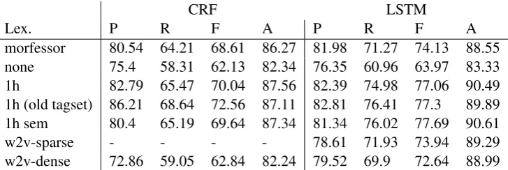
Table 1 contrasts the results of CRF and LSTM for different lexicalizations in “fast mode”. Re-markably, LSTM outperforms the CRF in all evaluation measures. A test with a higher-order CRF (not reported) shows that the accuracy of the CRF cannot be improved relevantly when wider ranges of output label transitions are considered, and increasing the range of input features also does not improve over the reported results.9 So, the deep NN seems to be more appropriate for this task than a CRF.
Comparing the previous large and the new smaller tagset yields consistent results for CRF and LSTM.10 While the previous tagset performs better for some low-frequency classes (higher F score),
the new tagset produces a higher overall accuracy, and requires less time for training due to its lower dimensionality. In addition, Table 1 demonstrates the high influence of the lexical representation. While the unlexicalized variant (none) suffers especially from low recall, the values ofmorfessorare clearly closer to the lexicalized than to the unlexicalized version, indicating that this approach may turn out to be useful for (ancient) Indian languages for which no extensive lexical resources, but large unannotated cor-pora are available. Finally, the variants using word embeddings (w2v-sparseand-dense) produce lower accuracy rates than the one-hot-encodings. Adding the broad word-semantic classes further improves the accuracy of the1hencoding, although the difference to1his not significant.
6The weight of a node is defined as the number of occurrences of the concept linked to the node, plus the sum of this number
for all its subnodes.
7Example: Although the node “mountain” has a very high weight, it is further collapsed into a parent node “elements of the
landscape”, which covers related concepts such as “lake” or “river”.
8Example: The subclasses of the concept “person” were widely scattered over the original tree and could, therefore, not be
subsumed automatically under one common ancestor.
9A first-order CRF with a feature window of 7 instead of 5 words producesP= 82.84,R= 64.13, andF = 68.71. 10Results for the tagset used in Hellwig (2015) have been recalculated for this paper using the same settings as for the other
CRF LSTM
Lex. P R F A P R F A
morfessor 80.54 64.21 68.61 86.27 81.98 71.27 74.13 88.55 none 75.4 58.31 62.13 82.34 76.35 60.96 63.97 83.33 1h 82.79 65.47 70.04 87.56 82.39 74.98 77.06 90.49 1h (old tagset) 86.21 68.64 72.56 87.11 82.81 76.41 77.3 89.89 1h sem 80.4 65.19 69.64 87.34 81.34 76.02 77.69 90.61
w2v-sparse - - - - 78.61 71.93 73.94 89.29
[image:6.595.118.482.62.184.2]w2v-dense 72.86 59.05 62.84 82.24 79.52 69.9 72.64 88.99
Table 1: Macro-average P(recision), R(ecall) and F(-score), and A(ccuracy) for all words with more than one morphological reading, “fast mode”. Note that macro-average measures tend to overemphasize (bad) results of small classes.
CRF LSTM
P R F A P R F A
[image:6.595.127.472.243.297.2]ambiguous 84.03 69.2 73.16 88.99 80.5 75.82 77.1 90.99 overall 90.46 79.68 82.62 95.17 87.36 83.11 84.5 96.01
Table 2: Macro-average PRF and accuracy on the full training set, features: 1h. First row: Results for ambiguous words; second row: Results for all words.
To make the results comparable with those reported for other languages, the second row of Table 2 reports the performance of the two models when trained with the 1h feature on the full data set. Remarkably, the CRF benefits more clearly from the increased training set, although its results are clearly worse than those of the LSTM.
Table 3, which splits the results of the best LSTM model from Table 1 according to coarse POS classes, confirms that the correct decisions were made when reducing the size of the tagset. The class of finite verbal forms, whose tense distinction strongly increased the size of the tagset, produce low error rates, while infinite declinable verbal forms are in a similar error range as adjectives and nouns.
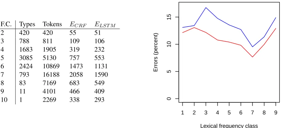
To obtain a more detailed error analysis, all instances misclassified by CRF or LSTM have been stratified according to binned frequency classes of their lemmata.11 The resulting data in Figure 1 allow
for two interesting observations. First, the performance of CRF and LSTM differs strongly with regard to frequency classes. Although the LSTM consistently outperforms the CRF in all frequency classes, the error rates of the two models differ by a nearly constant factor for low (classes 1 and 2) and high frequency words (classes 7-9). For the intermediate classes 3-6, the error rate of the LSTM decreases appproximately linearly with the frequency class, while the error rate of the CRF increases sharply for class 3, before decreasing for more frequent words. Note that class 3 is the first class for which lexical information is fed into both models.12 Contrary to the CRF, the LSTM seems to benefit from this
11The frequency class of wordwwith an observed frequencyNis given by the rounded value oflog(N)/log(5).
12Class 1 contains all hapax legomena, and class 2 words with corpus frequencies between 2 and 4 occurrences. As remarked
in Section 2.3, the experiments reported in Table 1 use a lexical frequency threshold of 5, such that class 3 is the first one for
POS A(dj.) I(nd.) N(oun) P(ron.) V.fin. V.inf. Acc. 92.4 100 95.73 93.4 99.58 94.1
F.C. Types Tokens ECRF ELST M
2 420 420 55 51
3 788 811 109 106
4 1683 1905 319 232
5 3085 5130 757 553
6 2424 10869 1473 1131 7 793 16188 2058 1590
8 83 7169 683 549
9 11 4101 466 409
10 1 2269 338 293 0
5
10
15
Lexical frequency class
Errors (percent)
[image:7.595.77.529.70.277.2]1 2 3 4 5 6 7 8 9
Figure 1: Number of lexical types and tokens, and of errors (ECRF, ELST M) per logarithmized
fre-quency class (F.C.; basis: 5). Right side: Percentual proportion of errors per frefre-quency class for CRF (blue) and LSTM (red). Models =1hfrom Table 1.
information right from the beginning.
The second observation concerns the high frequency classes 8 and 9, for which both classifier types produce increasing error rates. The majority of errors in these two frequency classes is caused by a small set of personal (tad‘he/she/it’, gender-neutralmad‘I’ andtvad‘you’), demonstrative (idam‘this’,
etad ‘this (here)’), and relative (yad ‘which’) pronouons, and by the quantifier sarva ‘all’, which is inflected like a pronoun. A closer inspection shows that ambiguities in case and gender assignment produce most of these errors. In 166 instances, for example, at least one of the models has made a wrong decision between N.SG.N. and A.SG.N. for one of the pronominal formstad,yad,etad, andidam, or for forms such asyasmin‘in which’, which can be analyzed either as masculine or as neuter of the locative singular. Some of the cases in which both models propose the same wrong analysis with high confidence values, actually give the correct reading of a misannotation in the corpus. Such results could be used for a future semi-automatic post-correction of the data.
Most of these errors, however, are caused by long-range constructions not detected by the model. The prose passage Vis.n.upur¯an.a 4.12.17 provides a – rather usual – example of such a complex construction, where the morphological disambiguation was not able to establish the correct link between the A.SG.N. -ratnamand its predecessor ending in-yugalam(only relevant morphological information given; words to be linked and their morphological information are underlined):
tasmim.´s
he:L.SG.M.
ca
and vidruterun away:L.SG.M. ’ti-tr¯asa-lola-¯ayata-locana-yugalam.very-fear-restless-extended-eye-pair:CO.. . . A.SG.N.
tr¯ahi
protect:imper.
tr¯ahi
protect
m¯am.
me t¯ata-ambafather-mother bhr¯atarbrother ityso agitated-lament-troubled:CO.-CO.-A.SG.N.¯akula-vil¯apa-vidhuram.
sa
he:N.SG.M.
r¯aja-kany¯a-ratnam
king-daughter-jewel:CO.-CO.-A.SG.N. adr¯aks.¯ıtsee:past, 3rd SG.
“After he (= a third person) had run away, he saw the jewel, which was the daughter of the king, whose pair of broad eyes was rolling due to (her) excessive fear, and which13was agitated by (her) confused
lament (stating) ‘Protect, protect me, o father, mother, brother’.” which lexical information is available.
Class P R F N.SG.N. 85.35 91.00 88.09 A.SG.N. 84.26 75.39 79.58 N.PL.M. 94.18 98.27 96.18 A.SG.M. 85.54 84.55 85.04 N.SG.M. 96.25 96.18 96.22 G.SG.M. 93.46 95.55 94.50 L.SG.N. 92.12 89.38 90.73 N.SG.F. 93.61 91.83 92.72 L.SG.M. 86.92 89.69 88.28 I.PL.M. 92.62 95.09 93.84 I.SG.M. 89.88 93.04 91.43
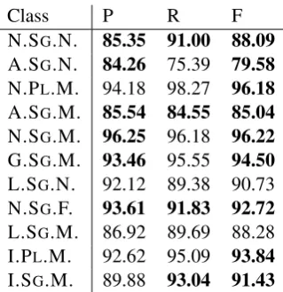
Table 4: P, R, and F of the full LSTM model for the most frequent nominal categories. Bold numbers are higher than the best results reported in Hellwig (2015). Note that the F score may be better than in Hellwig (2015), even if neither P nor R are better, because Hellwig (2015) considers these values for two models.
Each of the three compounds ending on-amcan be analyzed morphologically as N.SG.N., A.SG.N., or A.SG.M.. The morphological disambiguation has labeled the morphologically ambiguous compounds ending onvidhuramandratnamcorrectly as A.SG.N. This decision was probably supported by the fact that the pronoun sa‘he’ has only one morphological reading, and should therefore occupy the subject position of the singular verb, leaving the object slots free for the two accusative compounds. However, neither the LSTM nor the CRF were able to build the connection to thebahuvr¯ıhicompound ending on
-yugalamthat forms the opening bracket around the direct speech.
Contracted forms of gender neutral personal pronouns constitute another high-frequency and error prone group. The pronouns of the first (mad‘I’) and second person (tvad ‘you’) express their genitives and datives by morphologically unambiguous uncontracted (mama‘my’,mahyam‘for me’;tava‘your’,
tubhyam ‘for you’), and ambiguous contracted versions (me ‘my, for me’ and te‘your, for you’). In general, the use of dative and genitive becomes unstable in later and non-standard parts of the corpus, which may point to the linguistic influence of Middle and New Indo-Aryan languages. The passage R¯am¯ayan.a, Utt., 57.28, for example, uses the genitive to express the receiver in the verbal frame ofd¯a‘to give’: bhojanam . . . mama (G.SG.!) etad d¯atum icchasi“You want to give me this food.” The fact that the models are also trained on such non-standard instances may explain the high error rates for the contracted pronouns.
Table 4 presents precision, recall, and F scores for the most frequent morphological classes. Results are calculated from the output of the full LSTM model (Table 2). Comparing these values with the best results reported in Table 6 from Hellwig (2015) demonstrates that the LSTM clearly outperforms the published results, thereby setting a new standard for the morphological disambiguation of Sanskrit.
4 Conclusion
References
David Alfter and Jürgen Knauth. 2015. Morphological analysis and generation for Pali. InInternational Workshop on Systems and Frameworks for Computational Morphology. Springer, pages 60–71. Ronan Collobert, Jason Weston, Léon Bottou, Michael Karlen, Koray Kavukcuoglu, and Pavel Kuksa.
2011. Natural language processing (almost) from scratch. Journal of Machine Learning Research
12:2493–2537.
Mathias Creutz, Teemu Hirsimäki, Mikko Kurimo, Antti Puurula, Janne Pylkkönen, Vesa Siivola, Matti Varjokallio, Ebru Arisoy, Murat Saraçlar, and Andreas Stolcke. 2007. Morph-based speech recogni-tion and modeling of out-of-vocabulary words across languages. ACM Transactions on Speech and Language Processing (TSLP)5(1):1–27.
Mathias Creutz and Krista Lagus. 2007. Unsupervised models for morpheme segmentation and mor-phology learning. ACM Transactions on Speech and Language Processing4(1).
John Duchi, Elad Hazan, and Yoram Singer. 2011. Adaptive subgradient methods for online learning and stochastic optimization. Journal of Machine Learning Research12:2121–2159.
Jan Hajiˇc and Barbora Hladká. 1998. Tagging inflective languages: Prediction of morphological cat-egories for a rich, structured tagset. In Proceedings of the 36th Annual Meeting of the ACL. pages 483–490.
Oliver Hellwig. 2015. Morphological disambiguation of Classical Sanskrit. In Cerstin Mahlow and Michael Piotrowski, editors, Systems and Frameworks for Computational Morphology. Springer, Cham, pages 41–59.
Geoffrey E. Hinton, Nitish Srivastava, Alex Krizhevsky, Ilya Sutskever, and Ruslan R. Salakhutdinov. 2012. Improving neural networks by preventing co-adaptation of feature detectors. arXiv preprint arXiv:1207.0580.
Sepp Hochreiter, Yoshua Bengio, Paolo Frasconi, and Jürgen Schmidhuber. 2001. Gradient flow in recurrent nets: The difficulty of learning long-term dependencies. In S. C. Kremer and J. F. Kolen, editors,A Field Guide to Dynamical Recurrent Neural Networks.
Sepp Hochreiter and Jürgen Schmidhuber. 1997. Long Short-Term Memory. Neural Computation
9(8):1735–1780.
Gérard Huet. 2005. A functional toolkit for morphological and phonological processing, application to a Sanskrit tagger. Journal of Functional Programming15(04):573–614.
Gérard Huet. 2006. Lexicon-directed segmentation and tagging of Sanskrit. In B. Tikkanen and H. Het-trich, editors, Themes and Tasks in Old and Middle Indo-Aryan Linguistics, Motilal Banarsidass, Delhi.
Girish Nath Jha, Muktanand Agrawal, Sudhir K. Mishra, Diwakar Mani, Diwakar Mishra, Manji Bhadra, Surjit K. Singh, et al. 2009a. Inflectional morphology analyzer for Sanskrit. InSanskrit Computational Linguistics, Springer, pages 219–238.
Girish Nath Jha, Madhav Gopal, and Diwakar Mishra. 2009b. Annotating Sanskrit corpus: adapting IL-POSTS. InLanguage and Technology Conference. Springer, pages 371–379.
Sumitra M. Katre. 1991. Lexicography of Old Indo-Aryan: Vedic and Sanskrit. In Franz Josef Haus-mann, Oskar ReichHaus-mann, Herbert Ernst Wiegand, and Ladislav Zgusta, editors,Wörterbücher, Walter de Gruyter, Berlin, pages 2487–2496.
Amba Kulkarni and Devanand Shukla. 2009. Sanskrit morphological analyser: Some issues. Indian Linguistics70(1-4):169–177.
Tomáš Mikolov, Anoop Deoras, Daniel Povey, Lukáš Burget, and Jan ˇCernock`y. 2011. Strategies for training large scale neural network language models. In2011 IEEE Workshop on Automatic Speech Recognition and Understanding (ASRU). pages 196–201.
Anand Mishra. 2009. Simulating the P¯an.inian system of Sanskrit grammar. InSanskrit Computational Linguistics, Springer, pages 127–138.
Amr El-Desoky Mousa, M Ali Basha Shaik, Ralf Schlüter, and Hermann Ney. 2010. Sub-lexical lan-guage models for German LVCSR. InSpoken Language Technology Workshop (SLT). pages 171–176. S. Lakshmana Pandian and T. V. Geetha. 2009. CRF models for Tamil part of speech tagging and chunking. InProceedings of the 22nd International Conference on Computer Processing of Oriental Languages. Springer-Verlag, Berlin, Heidelberg, ICCPOL ’09, pages 11–22.
Richard Salomon. 1995. On drawing socio-linguistic distinctions in Old Indo-Aryan: The question of Ks.atriya Sanskrit and related problems. In George Erdosy, editor,The Indo-Aryans of Ancient South Asia. Language, Material Culture and Ethnicity, Walter de Gruyter, Berlin, New York, pages 293–306. Hartmut Scharfe. 1977.Grammatical Literature. A History of Indian Literature, Volume 5, Fasc. 2. Otto
Harrassowitz, Wiesbaden.