Comparing and combining classifiers for self-taught vocal interfaces
Lize Broekx, Katrien Dreesen, Jort F. Gemmeke, Hugo Van hamme
ESAT, KU Leuven, Leuven, Belgium
{katrien.dreesen,lize.broekx1}@student.kuleuven.be {jort.gemmeke,hugo.vanhamme}@esat.kuleuven.be
Abstract
An attractive approach to enable the use of vocal interfaces by impaired users with dysarthric speech is the use of a system which learns from the end-user. To enable such technology, it is imperative that the learning is fast to reduce the time spent train-ing the interface. In this paper we investigate to what extend various machine learning techniques are able to learn from only a single or a few spoken training samples. Additionally, we ex-plore whether these techniques can be combined through boost-ing to improve the performance. Our evaluations on a small, but highly realistic home automation database reveal that non-negative matrix factorization seems best suited for fast learning and that some of the boosting approaches can indeed improve performance, especially for small amounts of training data.
Index Terms: vocal user interface, self-taught learning, ma-chine learning, boosting
1. Introduction
Vocal user interfaces (VUIs) allow us to control a wide range of appliances and devices such as computers, smart phones, car navigation and other domestic devices and environments. While for most the use of a VUI is just a luxury, for individuals with a physical disability using a VUI can greatly improve their inde-pendence and quality of living, because for them operating and controlling devices would often require exhausting physical ef-fort [1].
Conventional speech recognition systems employed in VUIs are trained by the developer using vast amounts of speech material. While offering impressive performances for users whose word choice, grammar and speech conforms to the train-ing material used, performance suffers in the presence of ac-cented, dialectical and disordered speech. A possible solution, adaptation of existing acoustic models, may not suffice for se-vere speech pathologies [2, 3, 4, 5, 6].
The goal of this research is to explore methods which allow training speech commands by the end-user himself. This way, the acoustic models of the VUI are maximally adapted to the end-user’s speech while at the same time bringing development costs down. The challenge is to employ a learning strategy that can learn from only one or a few examples, in order to mini-mize the time the end-user spends on training the system. In this work, we will offer a comparison between multiple popu-lar machine learning strategies to evaluate their effectiveness in developing a fast learning self-taught VUI.
In previous work, we obtained encouraging results on fast vocabulary acquisition [7] using non-negative matrix factoriza-tion (NMF). Although in that work the learning speed of ac-quiring acoustic models was investigated, it focused on larger amounts of training data than targeted in this work. Moreover, it considered amulti-labeltask in which spoken utterances were
associated with multiple labels at once, which penalized other machine learning methods less suited for multi-label learning. In contrast, in this work we will focus onspeech classification, labelling a spoken utterance with a single label.
Our contribution is twofold. First, we compare the per-formance of five machine learning techniques: Dynamic Time Warping (DTW), Gaussian Mixture Models (GMMs), Hidden Markov Models (HMMs), Support Vector Machines (SVMs) and Non-negative Matrix Factorization (NMF). Each of these techniques have their strengths and weaknesses; for exam-ple, while a HMM improves upon a GMM by being able to model temporal structure, it does require more parameters to be trained. When training with only one or a few training samples, this may lead to overfitting. Second, we investigate to what extent combining the aforementioned classification techniques, ‘boosting’, can improve results. We do this by comparing a number of combination rules operating at the class label poste-rior level [8].
The remainder of the paper is organised as follows. In Sec-tion 2 we give an overview of the speech classificaSec-tion meth-ods that are investigated. In Section 3 we describe the various boosting approaches that will be considered. In Sections 4 and 5 we describe the experimental setup for evaluation on a small, but highly realistic home automation database collected in the ALADIN project [9]. The results of these experiments are pre-sented in Section 6 and discussed in Section 7, and we conclude with our summary and thoughts for future work in Section 8.
2. Classification methods
In a speech classification problem an unlabelled speech sig-nal X is assigned to one of the m possible commands {ω1, . . . , ωm}. The classification methods Dynamic Time
Warping (DTW), Gaussian Mixture Model (GMM) and Hidden Markov Model (HMM) use a spectrographic feature vector rep-resentationX= [x1, ...,xT]of a speech signalX, withT the
number of frames. The number of rows ofXis the dimension of the feature vectorxtfor one frame.
The classification methods Non-negative Matrix Factoriza-tion (NMF) and Support Vector Machine (SVM) use a utter-ance based feature vectorxof a speech signalX. The utterance based feature vectorxis a column vector whose dimensionN
depends on the kind of feature vector. More information about the feature vectors used in this work for each of the techniques is given in Section 4.2.
A classification method evaluates how well the unlabelled speech signal X resembles speech signals associated with a
command classωk. This similarity is expressed by the
posi-tive numberΠ(ωk, X), which is method dependent. The larger Π(ωk, X), the larger the similarity betweenX and the speech
as-signed to the commandωjwith the highest similarity:
assignX →ωj=argmax ωk
Π(ωk, X). (1)
2.1. Dynamic Time Warping
Dynamic Time Warping (DTW) [10, 11, 12], is a method in which an unlabelled speech signal is compared with a large col-lection of labelled speech signals (exemplars) extracted from the training data. Since such a comparison needs to take differ-ent signal lengths and speech rate variations into account, DTW first finds an optimal alignment between each pair of utterances through non-linear time warping. The unlabelled speech signal is labelled with the command which is associated with the most similar exemplar.
As a learning method, DTW has the advantage that it makes optimal use of all the available labelled data, because all train-ing samples can be used as an exemplar. A drawback of DTW is that the computational complexity of classification increases linearly with the number of training samples.
Formally, the similarity between the frames of the unla-belled speech signal X and the frames of each exemplarXi
is represented by aT ×Ti matrixDX,Xi containing the co-sine distance between the spectrographic based feature vectors representationsXandXi:
DX,Xi= X0Xi
kXkkXik
. (2)
The similarity between two speech signals is expressed as the scoreD˜X,X
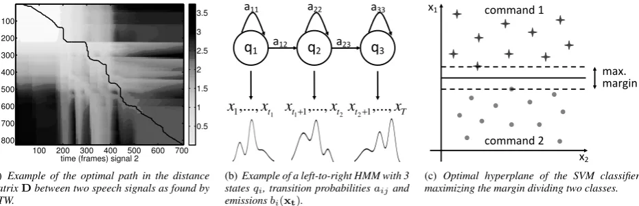
i along the optimal path through the distance matrixDX,Xi. The optimal path, from the left upper corner to the right lower corner (Figure 1(a)), minimises the cumulative acoustic differences and the total number of steps. The optimal path is determined using a dynamical programming approach with the Needleman-Wunsch algorithm [13].
The unlabelled speech signalXis assigned to the command of the exemplarXiwith the highest similarity. The similarity
betweenXandωkis expressed by the positive number
Π(ωk, X) = max Xiofωk
˜
DX,Xi. (3)
2.2. Gaussian Mixture Model
In a Gaussian Mixture Model (GMM), the probability density function is used to determine the acoustic likelihood of a com-mand given the feature vectors of the unlabelled speech signal [14].
Using a GMM is attractive, because it is a parametric model in which the classification of an unlabelled speech signal takes the same time independent of the amount of training data. An-other advantage is that the use of a parametric model typically allows better generalisation to unseen data, provided enough training data is available to accurately estimate the parameters.
Each command ωk is represented by a weighted sum of
multivariate Gaussian distributions
fk(xt,µ,Σ) = M
X
i=1
wiN(xt,µi,Σi), (4)
withµithe mean spectrographic based feature vector,Σithe
covariance matrix,withe weights for each multivariate
Gaus-sian distribution in the GMM andM the number of multivari-ate Gaussian distributions in the GMM. The weighted sum of multivariate Gaussian distributions for each command ωk is
trained on the collection of speech signals{X(1), . . . , X(N)} in the training data belonging to commandωk. By applying
the Expectation Maximization algorithm [15], the mean spec-trographic based feature vectorµi, the covariance matrixΣi
and the weightswiare obtained for each multivariate Gaussian
distribution in the GMM. The similarity betweenXandωkis
expressed by the positive number
Π(ωk, X) = exp 1
T
T
X
t=1
log (fk(xt,µ,Σ))
! . (5)
2.3. Hidden Markov Model
A Hidden Markov Model (HMM), the de facto standard model in automatic speech recognition, augments the GMM by taking the temporal structure of the speech into account.While known to be a powerful model for speech given enough training data, it is not clear a priori whether it can perform better than a GMM if there is very little training data and when whole-word HMMs to model the spoken commands are used rather than sub=words HMMs.
In a HMM for speech classification, the commandsωkare
represented by a sequenceQof statesq[16, 14]. For speech classification the order in the speech signal X is important, therefore a left-to-right (Bakis) HMM (Figure 1(b)) is used. A HMMλk= (Πk,Ak,Bk)is characterized by the initial
prob-abilitiesπ(ik), the transition probabilitiesa(ijk)and the emissions b(ik)(xt), whereiandjare the state indices. The emissionsBk
are a GMMfk(xt,µ,Σ)for each state.
The HMMλkis trained on the collection of speech signals
{X(1), . . . , X(N)}in the training data belonging to command
ωkby the Baum-Welch algorithm.
For an unlabelled speech signal X the optimal state se-quenceQ˜in each HMMλkis calculated as
˜
Q=arg max
Q P(Q|X, λk) =arg maxQ
P(Q,X|λk)
P(X|λk) . (6)
The similarity between X and ωk, which is obtained by
applying the Viterbi algorithm, is the positive number
Π(ωk, X) =P(X, q,|λk). (7)
2.4. Support Vector Machine
A Support Vector Machine is a linear classifier which is trained to be maximally discriminative between classes, possibly aug-mented by working in a high dimensional (kernalized) space [17]. SVMs are known to generalize well to unseen data, but it may be difficult to accurately train the hyperplane dividing classes with only few data points.
A SVM can be used for binary classification; to separate the
mcommands in our speech classification task we use the one-versus-one multi-label approach in this paper. For each pair of commandsωkandωl, a binary classification problem is solved,
which results innybinary classification problems with
ny=
m(m−1)
2 . (8)
The hyperplane of the linear classifier that separates two commandsωkandωlcan be formulated as
yωk,ωl(x) =w
T
time (frames) signal 2
ti
m
e
(
fr
a
m
e
s
)
s
ig
n
a
l
1
100 200 300 400 500 600 700 100
200
300
400
500
600
700
800
0.5 1 1.5 2 2.5 3 3.5
(a) Example of the optimal path in the distance matrixDbetween two speech signals as found by DTW.
1
,...,
1
x
tx
2 11
,...,
tt
x
x
+
x
t2+1,...,
x
Tq
1q
2q
3a11
a12
a22
a23
a33
(b)Example of a left-to-right HMM with 3 statesqi, transition probabilitiesaijand
emissionsbi(xt).
command 1
command 2 x1
x2
max. margin
[image:3.595.69.535.73.223.2](c) Optimal hyperplane of the SVM classifier maximizing the margin dividing two classes.
Figure 1:Graphical representation of the classification methods DTW, HMM and SVM.
withwωk,ωl ∈R
n, x
∈Rn, b
ωk,ωl ∈R, yωk,ωl ∈R. The unique hyperplane for a binary classification problem (Figure 1(c)) can be found by rescaling the problem such that the x closest to the hyperplane satisfy
|wωk,ωl
Tx+b
ωk,ωl|= 1. (10)
The speech signalXis associated with label vector
y(x) = [yω1,ω2(x), . . . , yωm−1,ωm(x)]
T, (11)
withxthe utterance based feature vector ofX.
Each commandωkis associated with a command label
vec-tory(k)
∈ {−1,+1}ny. The similarity between the speech signalXand commandωkis the positive number
Π(ωk, X) =
y(k)==sign(y(x)). (12)
2.5. Non-negative Matrix Factorization
Non-negative Matrix Factorization is an approach which fac-torises the training data into a set of recurrent acoustic patterns and their activations. In a supervised setting, these acoustic pat-terns take on the distribution of the spoken commands, as well as the acoustic patterns of filler words which are shared between commands, e.g. the, and, please. As such, it can potentially leverage shared information between commands.
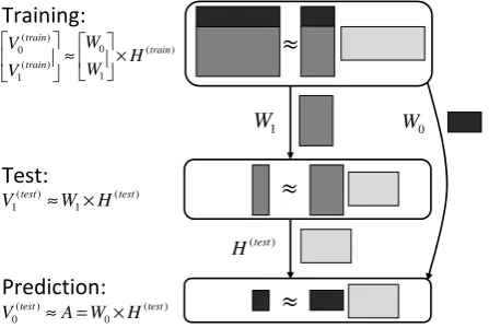
A scheme of the Non-negative Matrix Factorization (NMF) is given in Figure 2 [18]. The non-negative matrixV(train) con-sists of two parts, viz. [V0(train);V1(train)]. Each of them
com-mandsωkis represented by a vector representationy(k), which
is a zero mdimensional vector with a 1 on positionk. The columns of the matrixV0(train)contain the vector representation
y(k)of the commandω
kfor each utterance in the training data,
soV0(train)is a matrix of dimensionm×Ntrain. The columns of the matrixV1(train)contain the utterance based feature vectorx
for each utteranceXin the training data, soV1(train)is a matrix
of dimension length(x)×Ntrain. A low rank representation for V1(train)is obtained by factorizingV(train)as the product of two
non-negative matricesWandH(train), viz.
V0(train)
V1(train)
≈
W0
W1
H(train)=WH(train). (13)
The number of columns ofW, i.e. the number of acoustic patterns to extract from the training data, is fixed in advance.
The matricesW andH(train) are obtained by iteratively min-imizing the Kullback-Leibler divergence [19] betweenV(train) and WH(train). After training, the matrix W1 contains as
columns the acoustic patterns that exist in the training data. El-ementW0(k, j)indicates if the acoustic pattern in columnj
ofW1 is present in commandωk. The elementH(train)(i, j)
indicates how much the acoustic pattern in column iof W1
is present in utteranceX(j) of the training data (columnjof V1(train)).
For speech classification with NMF, the utterance based feature vector x of speech signal X is used as vector
V1(test). By minimizing the Kullback-Leibler divergence
be-tweenV1(test)andW1H(test), the vectorH(test)is calculated
V1(test)≈W1H(test). (14)
An approximation ofV0(test), containing the representation
of the command for each utterance in the test data, is given by the activation vectorA
V0(test)≈A=W0H(test). (15)
The similarity between speech signalXand commandωk
is given by the positive number
Π(ωk, X) =A(k). (16)
3. Combining methods
Each classification method uses different mechanisms to assign an unlabelled speech signalX to the most probable command
ωj. As a result, not all classification methods assign an
unla-belled speech signal to the same command, so the misclassifi-cations differ. In this paper we investigate whether combiningR
different classification methods, i.e. boosting [8], might reduce the number of misclassifications. Each methodr calculates a positive numberΠr(ωk, X)for each commandωk.
The numbers{Πr(ωk, X)}Mk=1are normalized to construct a probability vectorprfor each method. The combination of
the classification methods assigns the unlabelled speech signal
Xto the commandωjwith the highest a posteriori probability
assignX→ωj=argmax ωk
P(ωk|p1, ...,pR). (17)
Figure 2:Scheme of Non-negative Matrix Factorization.
) (
1 0 ) ( 1
) (
0 train
train train
H W W V
V
×
≈
0 W 1
W
) ( 1 ) ( 1
test test
H W
V ≈ ×
) (test
H
) ( 0 ) ( 0
test test
H W A V ≈ = ×
Training:
≈
≈
≈
Test:
Prediction:
The combination rules in Table 1 make the assumption that each method assigns a speech signal to a command indepen-dently of the other methods, which results in
P(p1, ...,pR|ωk) = R
Y
i=1
P(pi|ωk). (18)
In this paper the extra assumption of equal a priori probabili-ties is made for each rule. The a posteriori probability of the product rule is obtained by repeatedly applying Bayes’ rule. In the sum rule the assumption is made that the a posteriori prob-abilitiesP(ωk|pi)calculated by the different methods do not
significantly differ from the a priori probabilitiesP(ωk). The maximum rule is obtained starting from the sum rule and using the relation
1
R
R
X
i=1
P(ωk|pi)≤max
i P(ωk|pi). (19)
The minimum rule is obtained starting from the product rule and using the relation
R
Y
i=1
P(ωk|pi)≤min
i P(ωk|pi). (20)
The a posteriori probability of the median rule is obtained by replacing the mean by the more robust median in the sum rule. In the majority rule the assumption is made that the a posteriori probabilitiesP(ωk|pi)calculated by the different methods do
not significantly differ from the a priori probabilitiesP(ωk).
4. Experimental setup
4.1. DatasetThe experiments are performed on the first home automation dataset (DOMOTICA-1) of the ALADIN project [9]. The dataset
consists of non-pathological speech commands which were recorded in a realistic setting, i.e. a fully automated room using a wizard-of-oz device control. The commands were prompted using visual cues (a video) on a computer screen. In order to simulate situations with environmental noise, recordings were also made with a concurrent sound source. In addition to a close-talk microphone, multichannel audio recordings were made with multiple microphone arrays, placed near the user, on walls and near the optional noise source.
Table 1: A posteriori probabilities for combination rules in assumption of equal a priori probabilities.
rule P(ωk|p1, ...,pR)
product
R
Y
i=1
P(ωk|pi)
sum
R
X
i=1
P(ωk|pi)
maximum max
i P(ωk|pi)
minimum min
i P(ωk|pi)
median med
i P(ωk|pi)
majority 1
R
R
X
i=1
∆k,i
with∆k,i=
(1 ifω
k=argmax ωl
P(ωl|pi)
0 otherwise
The noisy recordings were created by playing a radio in the background with a sound level of 60dB Sound Pressure Level, which is the sound level of average speech. It was ensured that the measured SNR to the nearest microphone remained above 15dB.
The dataset consists of 27 test subjects of which 20 are of the targeted user group. Each person was asked to go repeatedly through a list of 33 different actions, until a recording time of 30 minutes was reached, yielding a dataset of1888commands for the target group. In addition to this set, longer recording sessions with7non-target users were carried out, yielding1699
spoken commands.
The experiments are performed on persons 5,7,20,22 and 26, on the noisy dataset recorded with the close-talk micro-phone. These speakers were selected because they were the only speakers with at least 3 spoken samples of each command. We will refer to them by these numbers to keep correspondence with other work on the same dataset.
4.2. Acoustic representation
In this paper two classes of feature vectors are used: spectro-graphic based feature vectors and utterance based feature vec-tors [20, 21]. The MFCC, MFCCDD and MIDA feature vecvec-tors are used as spectrographic based feature vectors. The GMM-supervector and the feature vector based on the histogram of acoustic occurrences and co-occurrences (sumHAC) are used as utterance based feature vector [18]. In this paper a Hamming window of size 30 ms is used with frame shifts of 15 ms. A pre-emphasis of 0.95 is used.
The MFCC feature vectors are obtained by applying an In-verse Discrete Cosine Transform (IDCT) to log-Mel spectra. In this paper, we use 12 MFCCs in each frame, in addition to the log energy, resulting in 13-dimensional feature vectors. To ob-tain the MFCCDD feature vectors, the 13-dimensional MFCC feature vectors are augmented with their first and second order differences (∆- and∆∆-features), yielding a total of 39 coeffi-cients per frame.
The Mutual Information Discriminant Analysis (MIDA) feature vectors are obtained with a linear transformation that maximizes the separability between different classes of input frames [22]. In this paper, we determine∆- and∆∆-features
[image:4.595.313.540.108.276.2]input vectors. On these representations we then perform the MIDA-transformation, separating the classes in the input space and at the same time reducing its dimensionality from 72 to 39. The spectrographic based feature vectors are the starting point to construct the utterance based feature vectors. The GMM-supervector combines 60-dimensional MFCCDD spec-trographic based feature vectors to one high-dimensional utter-ance based feature vector [21]. The construction of a GMM-supervector consists of three steps. The first step is training a Gaussian Mixture Model Universal Background Model (GMM UBM). To be more robust, a trained GMM UBM with 512 mul-tivariate Gaussian distributions is used. The development data set used to train the UBM includes over 30,000 speech record-ings and was sourced from NIST 2004-2006 SRE databases, LDC releases of Switchboard 2 phase III and Switchboard Cel-lular (parts 1 and 2) [23]. The second step in constructing a GMM-supervector is adapting the means of the multivariate Gaussian distributions of the GMM UBM according to the spec-trographic based feature vectors of the speech signal. In the last step the 512 adapted means of dimension 60 are placed in a column vector, which gives the resulting 30720-dimensional GMM-supervector of the speech signal.
The utterance based feature vector based on the histogram of acoustic occurrences and co-occurrences (sumHAC) is con-structed by applying a k-means clustering algorithm [16] to the MFCCDD spectrographic based feature vectors to obtain a codebook [18]. Each spectrographic based feature vector is assigned to a prototype vector in the codebook by means of an extension (softVQ) to vector quantization [24]. With softVQ a frame based feature vector characterized by its proximity to multiple prototypes is obtained. Proximity is measured as the posterior probability of a collection of Gaussians, much like in semi-continuous HMMs.
In this paper Voice Activity Detection (VAD) is used to improve the performance of a classification method [25]. By distinguishing speech and silence frames in the speech signal, both training and classification are only based on the speech frames. The distinction between speech and silence frames is made based on the energy in the frame.
4.3. Classification methods
Below, we detail the acoustic representations and parameter set-tings for each of the methods. To ensure a best-case scenario for each of the methods, we optimised the settings for each method individually.
DTW employs MFCC feature vectors. The use of MFC-CDD and MIDA features was explored in a pilot experiment, but did not result in significant improvements.
Both the GMM and the HMM use the spectrographic MIDA feature vectors. The full-covariance GMM consists of 10 mix-tures, while the GMM employed in the HMM uses 5 mixtures and a three state left-to-right HMM. The implementation uses the logarithm of the probabilities to obtain a numerically stable implementation [26].
The linear kernel SVM operates on GMM-supervectors, tuned using a cross-validation grid search. Finally, NMF is applied to the utterance based feature vector sumHAC, con-structed starting from the spectrographic based feature vector MFCCDD and using the vector quantization method softVQ. In this paper codebooks of size 50 are used for softVQ and 36 acoustic patterns are extracted from the training data (columns ofW), where 3 are used for filler words.
Table 2 gives an overview of the setting for the different
Table 2: Settings for each classification method.
method setting
DTW MFCC
GMM MIDA, 10 mixtures
HMM MIDA, 3 states, 5 mixtures
SVM GMM-supervector (MFCCDD)
NMF sumHAC (MFCCDD, softVQ)
classification methods.
5. Experiments
5.1. Comparing classifiersFor the experiment to determine the best classification method only 22 commands with 3 examples or more in the noisy record-ing scenario of person 5, 7, 20, 22 and 26 are considered. There is not enough data for the other persons in the data to investigate the influence of the number of examples for each command on the classification.
In a small dataset, the division of the commands in groups with cross-validation is more important than in larger datasets. Therefore an adaptation of cross-validation is used in the exper-iments. The commands are randomly divided in groups with the requirement that in each group there is exactly one speech sig-nal belonging to each command. The least frequent command in the dataset determines the number of disjunct groups. The remaining speech signals are not used in the experiments.
To determine the accuracies of the different classification methods forkexamples for each command, the classification methods are trained onkdisjunct groups and tested on 1 dis-junct group. All possible combinations of training groups and test group are considered. To minimize the influence of the di-vision in groups, the experiments are repeated with 5 different random divisions in groups.
5.2. Combining classifiers
For the experiment to determine the influence of boosting on the accuracy only 22 commands with 3 examples or more in the noisy dataset of person 26 are considered. For each method
i∈ {DTW, GMM, HMM, SVM, NMF}the22×22matrixΠi
is constructed with as(k, j)element the numberΠi(ωk, X(j))
whereωk is the considered command andX(j)a speech
sig-nal in the testdata. Each column in the matrix Πi is scaled
to a probability vector, resulting in the matrixPi. The
adap-tation of cross validation, as discussed in section 5.1, is used and the experiments are repeated with 5 different random di-visions in groups to minimize the influence of the division in groups. The matricesPiof the different combinations of test
group and trainingsdata with 5 random divisions in groups are concatenated in the matrixPi,TOTfornexamples in the train-ingsdata. The matrixPi,TOTis of dimension22×NTOT, where
NTOTis the product of the number of commands (22), the num-ber of random divisions in groups (5), the numnum-ber of test groups and the number of different trainingsdata fornexamples in the trainingsdata.
The goal of boosting is to achieve an improvement in the accuracies with respect to the individual classification methods. In the boosting experiment, each methodiis assigned a
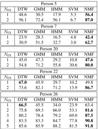
Table 3:Accuracies obtained with classification methods in noisy recording scenario for person 5, 7, 20, 22 and 26.
Person 5
NEX DTW GMM HMM SVM NMF
1 48.6 30.5 17.9 5.3 56.4
2 56.1 72.4 56.1 6.7 87.0
Person 7
NEX DTW GMM HMM SVM NMF
1 23.9 28.3 16.5 4.8 42.4
2 30.9 51.5 32.7 3.0 62.7
Person 20
NEX DTW GMM HMM SVM NMF
1 45.0 47.3 29.2 10.8 47.6
2 54.8 71.2 55.8 30.6 80.0
Person 22
NEX DTW GMM HMM SVM NMF
1 67.0 45.9 29.7 10.2 49.8
2 73.6 82.1 71.2 13.9 86.7
Person 26
NEX DTW GMM HMM SVM NMF
1 66.5 45.5 34.0 23.9 63.4
2 75.8 69.3 66.0 53.1 81.6
3 80.2 78.4 79.2 69.0 87.5
4 83.5 83.3 84.7 77.8 90.8
5 85.6 85.9 88.2 81.5 91.8
majority rule the definition of∆k,ibecomes
∆k,i=
(w
i ifωk=argmax ωl
P(ωl|pi)
0 otherwise. (21)
In this way a better classification method has a higher influence on the a posteriori probability.
The optimal weightswiof the matricesPi,TOTof the meth-ods i in the boosting rules are obtained using grid search for 1 example for each command. The grid search of the weight wi for each methodi is between 0 and 1 with step
size 1/4. Each possible combination of the weights w = [wDTW, wGMM, wHMM, wSVM, wNMF] is scaled to one. For the combination rules, the weightsw = [1/4,1/4,1/4,1/4,1/4]
andw = [1,1,1,1,1]result in the same normalized weights w = [1/5,1/5,1/5,1/5,1/5]. Only the unique normalized
weights are considered. If there are multiple weightswwhich result in the highest accuracies, the firstwis used as optimal weight.
6. Results
6.1. Comparing classifiersTable 3 shows the accuracies with differentNEXexamples for each command in the trainingsdata and for person 5, 7, 20, 22 and 26 with the settings of Table 2.
Table 3 shows that NMF gives the highest accuracies for each person, except for person 22 and 26 with one example for each command. The lowest accuracies are obtained with classification method SVM. The accuracies improve with an in-creasing number examplesNEXfor each command, except for person 7 with SVM. The accuracies of person 7 are significantly lower than those of the other persons. For person 5 the second highest accuracies are obtained with DTW and NMF for 1 and
Table 4: Weights for person 26 with combination rules.
rule DTW GMM HMM SVM NMF
product 4/5 0 0 0 1/5
sum 4/5 0 0 0 1/5
maximum 4/5 0 0 0 1/5
minimum 1/17 4/17 4/17 4/17 4/17
median 1/6 4/6 0 0 1/6
majority 2/6 1/6 0 1/6 2/6
Table 5: Accuracies for person 26 with combination rules.
NEX product sum max min med maj
1 73.0 70.6 70.7 23.9 66.7 70.2
2 85.2 83.8 83.5 52.7 79.3 83.4
3 89.3 88.8 87.8 68.7 84.4 88.3
4 91.2 91.0 90.6 77.5 88.2 90.8
5 92.9 92.0 91.1 81.2 90.5 91.7
2 examples for each command respectively. For person 7 and 20 the second highest accuracies are obtained with GMM. The second highest accuracies for person 22 are obtained with NMF (1 example) and GMM (2 examples). For person 26 the second highest accuracies are obtained with NMF (1 example), DTW (2-3 examples) and HMM (4-5 examples). The accuracies of person 26 with GMM are initially higher than those of HMM (1-2 examples), but for more examples (3-5) the accuracies of HMM are higher.
6.2. Combining classifiers
In Table 4 the optimal weights are shown that are obtained by grid search with 1 example for each command in the training data.
Table 4 shows that the product rule, sum rule and maximum rule assign an unlabelled speech signalX based on the
proba-bility vectorspDTW andpNMF. The median rule uses the
probability vectorspDTW,pGMMandpNMF. The majority
rule uses all probability vectors exceptpHMM. The minimum
rule bases the assignment on the probability vectors of all classi-fication methods. The according non normalized weights in the grid search arew = [1/4,1,1,1,1]. In the minimum rule the probability vectorpDTWgets the smallest weight. In Table 5
the accuracies obtained with the individual classification meth-ods and the different boosting rules with weights as in Table 4 are shown.
Table 5 shows that the highest individual accuracies are ob-tained with the classification method DTW (1 example) and NMF (2-5 examples). The classification method SVM gives the lowest accuracies. The more examples for each command in the training data, the higher the accuracies of the individual classification methods are.
are lower than the accuracies obtained with the best individ-ual classification method NMF, except for 1 example for each command. The median rule performs better than all individual classification methods except NMF. The minimum rule gives similar accuracies as the worst individual classification method SVM.
7. Discussion
7.1. comparing classifiersWhen comparing the classifiers in Table 3, we observe a very large difference between classification methods. Since for speaker 26, the difference between methods becomes substan-tially smaller with increasing numbers of examples per com-mand, we can indeed attribute most of these difference to the amount of training data used. Although it is difficult to set a tar-get accuracy which suffices for practical applicability of these techniques, it is encouraging that for most speakers 2 examples suffice to achieve 80 to 90 % accuracy. The lower accuracies of speaker 7, although still at 62.7 % for NMF, are due to a speech impairment. Informal listening tests revealed that for this speaker, the spoken commands are difficult to understand even for humans.
As expected, DTW achieves good results when presented with only a single training sample, but is outperformed by mod-els which learn their parameters as soon as there is more training data. It is interesting to observe that HMM is outperformed by the simpler GMM until at least 3 training samples are presented. It seems that even though the GMM employed by the HMM is smaller (5 vs 10 mixtures), the larger number of parameters that needs to be trained is still problematic for small training sizes.
Of all the methods, the SVM performs the worst, with re-sults almost at chance level for some speakers. The rere-sults on speaker 26 indicate once again, that with more data the results become comparable. NMF, on the other hand, is able to per-form well both with little and larger amounts of training data. Presumably, this is due to its capability to use some of its recur-rent patterns to model phenomena such as filler words, which allows the recurrent patterns modelling commands to be more discriminative. Although these results do not allow us to inves-tigate the accuracy when presented with much more data (hun-dreds of examples), but results in [7] do indicate that also in these regimes, NMF be adequate.
7.2. Combining classifiers
Unfortunately, the amount of data available did not allow us to explore methods which learn the boosting weights from the data. Our experiments therefore show an upper limit on the performance gains that can be expected using boosting. Addi-tionally, the weights that are obtained allow us to judge which methods offer complementary information.
The product rule, sum rule and maximum rule only use the 2 classification methods DTW and NMF which have the highest accuracies for 1 example for each command. The weightwDTW is higher thanwNMF because the accuracy of DTW is higher than that of NMF for 1 example for each command. Since these rules have the highest weight to the best classification method, the best accuracies are obtained for these rules in comparison with the other boosting rules. This effect is only visible for a few examples for each command. An explanation for this is that the best classification method DTW for 1 example gains little in comparison with the other classification methods when increasing the amount of examples for each command.
The accuracies obtained with the minimum rule are not more than the accuracies obtained with the worst classification method SVM. It is plausible that the minimum rule only gives good results if the entropy of the probabilities of the different commands for the classification methods is small (probabilities of different commands in one classification method are close together). This is not the case for the considered classification methods. In this experiment, the minimum rule has the opposite effect of what is expected of a boosting rule.
The median rule does not take the classification method HMM and SVM, which have the lowest accuracies for 1 exam-ple for each command. The obtained accuracies are similar to the accuracies obtained with NMF. This is achieved by giving the best classification methods NMF and DTW a weight such that their weighted probability vector is median.
The majority rule assigns a relative high weight to the 2 best classification methods DTW and NMF for 1 example for each command, as expected. GMM and SVM also get a non zero weight. HMM is assigned a zero weight, which is explained by the fact that HMM makes more and similar misclassifications than GMM, because of the lack of data for 1 example for each command.
The effect of boosting decreases when increasing the amount of examples for each command. This is explained by the weights are trained on 1 example for each command and the changing order of best classification methods. Some classifica-tion methods (HMM, SVM) need more data to obtain a higher accuracy, while DTW gains relatively little in accuracy when increasing the number of data.
8. Conclusions
In this paper the performance of the classification methods Dynamic Time Warping (DTW), Gaussian Mixture Model (GMM), Hidden Markov Model (HMM), Support Vector Ma-chine (SVM) and Non-negative Matrix Factorization (NMF) are investigated on a speech classification task. Evaluations on a re-alistic home automation database show that NMF is best suited for speech classification with a small amount of data. Next, we investigated if combining different methods through boosting might improve the classification. Both the product rule and the sum rule give higher accuracies than the best individual classi-fication method. The gain of combining classiclassi-fication methods is higher for a small amount of data. Future work will focus on exploring methods to learn the boosting weights on small amounts of training data.
9. Acknowledgements
The research of Jort F. Gemmeke is funded by IWT-SBO grant 100049.
10. References
[1] J. Noyes and C. Frankish, “Speech recognition technology for
in-dividuals with disabilities,”Augmentative and Alternative
Com-munication, vol. 8, no. 4, pp. 297–303, 1992.
[2] H. Christensen, S. Cunningham, C. Fox, P. Green, and T. Hain, “A comparative study of adaptive, automatic recognition of
disor-dered speech,” inProc Interspeech 2012, Portland, Oregon, US,
Sep 2012.
[3] K. T. Mengistu and F. Rudzicz, “Comparing humans and au-tomatic speech recognition systems in recognizing dysarthric
speech,” inProceedings of the Canadian Conference on Artificial
[4] H. V. Sharma and M. Hasegawa-Johnson, “State transition in-terpolation and map adaptation for hmm-based dysarthric speech
recognition,” inHLT/NAACL Workshop on Speech and Language
Processing for Assistive Technology (SLPAT), 2010, pp. 72–79. [5] F. Rudzicz, “Acoustic transformations to improve the
intelligibil-ity of dysarthric speech,” inProceedings of the Second Workshop
on Speech and Language Processing for Assistive Technologies (SLPAT2011), 2011.
[6] M. S. Hawley, P. Enderby, P. Green, S. Cunningham, S. Brownsell, J. Carmichael, M. Parker, A. Hatzis, P. O’Neill, and R. Palmer, “A speech-controlled environmental control system for
people with severe dysarthria,”Medical Engineering & Physics,
vol. 5, no. 29, pp. 586 – 593, 2007.
[7] J. Driesen, J. Gemmeke, and H. Van hamme, “Weakly super-vised keyword learning using sparse representations of speech,” inProceedings of the 36th International Conference on Acoustics, Speech and Signal Processing, Kyoto, Japan, 2012.
[8] J. Kittler, M. Hatef, R. P. W. Duin, and J. Matas, “On
combin-ing classifiers,”Pattern Analysis and Machine Intelligence, IEEE
Transactions on, vol. 20, no. 3, pp. 226–239, 1998.
[9] ALADIN, “Adaptation and Learning for
Assis-tive Domestic Vocal INterfaces,” Project Page:
http://www.esat.kuleuven.be/psi/spraak/projects/ALADIN. [10] T. N. Sainath, B. Ramabhadran, D. Nahamoo, D. Kanevsky, D. V.
Compernolle, K. Demuynck, J. F. Gemmeke, J. R. Bellegarda, and S. Sundaram, “Exemplar-based processing for speech
recog-nition,”IEEE Signal Processing Magazine, vol. 29, no. 6, pp. 98–
113, 2012.
[11] D. Ellis, “Dynamic Time Warp (DTW)
in Matlab,” Web resource, available:
http://www.ee.columbia.edu/ dpwe/resources/matlab/dtw/,
2003.
[12] M. De Wachter, M. Matton, K. Demuynck, P. Wambacq, R. Cools, and D. Van Compernolle, “Template-based continuous speech
recognition,” Audio, Speech, and Language Processing, IEEE
Transactions on, vol. 15, no. 4, pp. 1377–1390, 2007.
[13] S. B. Needleman and C. D. Wunsch, “A general method applicable to the search for similarities in the amino acid sequence of two
proteins,”Journal of molecular biology, vol. 48, no. 3, pp. 443–
453, 1970.
[14] D. Jurafsky and J. H. Martin,Speech and language processing: an
introduction to natural language processing, computational lin-guistics and speech recognition, 2nd ed. Pearson International Edition, 2009.
[15] S. K. Ng, T. Krishnan, and G. J. McLachlan, “The EM algorithm,”
Handbook of computational statistics, vol. 1, pp. 137–168, 2004.
[16] X. Huang, A. Acero, H.-W. Honet al.,Spoken language
process-ing. Prentice Hall PTR New Jersey, 2001, vol. 15.
[17] J. A. K. Suykens, T. Van Gestel, J. De Brabanter, B. De Moor, and
J. Vandewalle,Least Squares Support Vector Machines. World
Scientific Publishing Co. Pte. Ltd., 2002.
[18] J. Driesen, “Discovering words in speech using matrix factoriza-tion,” Ph.D. dissertation, Ph. D. dissertation, KU Leuven, ESAT, 2012.
[19] T. M. Cover and J. A. Thomas,Elements of information theory.
Wiley-interscience, 2012.
[20] J. Driesen, J. F. Gemmeke, and H. Van hamme, “Data-driven
speech representations for NMF-based word learning,” inProc.
SAPA-SCALE, 2012, pp. 98–103.
[21] M. H. Bahariet al., “Speaker age estimation using Hidden Markov
Model weight supervectors,” inInformation Science, Signal
Pro-cessing and their Applications (ISSPA), 2012 11th International Conference on. IEEE, 2012, pp. 517–521.
[22] K. Demuynck, J. Duchateau, and D. Van Compernolle, “Opti-mal feature sub-space selection based on discriminant analysis,” inProc. Eurospeech, vol. 3, 1999, pp. 1311–1314.
[23] M. H. Bahari, R. Saeidi, H. Van hamme, and D. van Leeuwen, “Accent recognition using i-vector, gaussian mean supervector and gaussian posterior probability supervector for spontaneous
telephone speech,”Proceedings ICASSP 2013, 2013.
[24] S. Meng and H. Van hamme, “Coding Methods for the NMF Ap-proach to Speech Recognition and Vocabulary Acquisition,” 2011. [25] J. Ramirez, J. M. G´orriz, and J. C. Segura, “Voice activity de-tection. fundamentals and speech recognition system robustness,”
Robust Speech Recognition and Understanding, pp. 1–22, 2007. [26] T. P. Mann, “Numerically stable hidden Markov model