Investigating Content Selection for Language Generation using Machine Learning

Investigating Content Selection for Language Generation using Machine

Learning

Colin Kelly Computer Laboratory University of Cambridge

15 JJ Thomson Avenue Cambridge, UK

Ann Copestake Computer Laboratory University of Cambridge

15 JJ Thomson Avenue Cambridge, UK

{colin.kelly,ann.copestake,nikiforos.karamanis}@cl.cam.ac.uk Nikiforos Karamanis Department of Computer Science

Trinity College Dublin Dublin 2

Ireland

Abstract

The content selection component of a nat-ural language generation system decides which information should be communi-cated in its output. We use informa-tion from reports on the game of cricket. We first describe a simple factoid-to-text alignment algorithm then treat content se-lection as a collective classification prob-lem and demonstrate that simple ‘group-ing’ of statistics at various levels of granu-larity yields substantially improved results over a probabilistic baseline. We addi-tionally show that holding back of specific types of input data, and linking database structures with commonality further in-crease performance.

1 Introduction

Content selection is the task executed by a natu-ral language generation (NLG) system of decid-ing, given a knowledge-base, which subset of the information available should be conveyed in the generated document (Reiter and Dale, 2000).

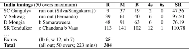
Consider the task of generating a cricket match report, given the scorecard for that match. Such a scorecard would typically contain a large num-ber of statistics pertaining to the game as a whole as well as individual players (e.g. see Figure 1). Our aim is to identify which statistics should be selected by the NLG system.

Much work has been done in the field of con-tent selection, in a diverse range of domains e.g. weather forecasts (Coch, 1998). Approaches are usually domain specific and predominantly based on structured tables of well-defined input data.

Duboue and McKeown (2003) attempted a sta-tistical approach to content selection using a sub-stantial corpus of biographical summaries paired with selected content, where they extracted rules

and patterns linking the two. They then used ma-chine learning to ascertain what was relevant.

Barzilay and Lapata (2005) extended this ap-proach but applying it to a sports domain (Amer-ican football), similarly viewing content selection as a classification task and additionally taking ac-count of contextual dependencies between data, and found that this improved results compared to a content-agnostic baseline. We aim throughout to extend and improve upon Barzilay and Lapata’s methods.

We emphasise that content selection through statistical machine learning is a relatively new area – approaches prior to Duboue and McKeown’s are, in principle, much less portable – and as such there is not an enormous body of work to build upon.

This work offers a novel algorithm for data-to-text alignment, presents a new ‘grouping’ method for sharing knowledge across similar but distinct learning instances and shows that holding back certain data from the machine learner, and rein-troducing it later on can improve results.

2 Data Acquisition & Alignment

We first must obtain appropriately aligned cricket data, for the purposes of machine learning.

Our data comes from the online Wisden al-manack (Cricinfo, 2007), which we used to down-load 133 match report/scorecard pairs. We em-ployed an HTML parser to extract the main text from the match report webpage, and the match data-tables from the scorecard webpage. An ex-ample scorecard can be found in Figure 11.

1

Cricket is a bat-and-ball sport, contested by two oppos-ing teams of eleven players. Each side’s objective is to score more ‘runs’ than their opponents. An ‘innings’ refers to the collective performance of the batting team, and (usually) ends when all eleven players have batted.

ResultIndia won by 63 runs

India innings(50 overs maximum) R M B 4s 6s SR

SC Ganguly∗ run out (Silva/Sangakarra†) 9 37 19 2 0 47.36

V Sehwag run out (Fernando) 39 61 40 6 0 97.50

D Mongia b Samaraweera 48 91 63 6 0 76.19

SR Tendulkar c Chandana b Vaas 113 141 102 12 1 110.78

. . .

Extras (lb 6, w 12, nb 7) 25

Total (all out; 50 overs; 223 mins) 304

Fall of wickets1-32 (Ganguly, 6.5 ov), 2-73 (Sehwag, 11.2 ov), 3-172 (Mongia, 27.4 ov), 4-199 (Dravid, 32.1 ov), . . . , 10-304 (Nehra, 49.6 ov)

Bowling O M R W Econ

WPUJC Vaas 10 1 64 1 6.40 (2w)

DNT Zoysa 10 0 66 1 6.60 (6nb, 2w)

. . .

TT Samaraweera 8 0 39 2 4.87 (2w)

Figure 1: Statistics in a typical cricket scorecard.

2.1 Report Alignment

We use a supervised method to train our data, and thus need to find all ‘links’ between the scorecard and match report. We execute this alignment by first creating tags with tag attributes according to the common structure of the scorecards, and tag values according to the data within a particular scorecard. We then attempt to automatically align the values of those tags with factoids, single pieces of information found in the report.

For example, from Figure 1 the fact that Ten-dulkar was the fourth player to bat on the first team is captured by constructing a tag with tag attribute

team1 player4, and tag value ‘SR Tendulkar’. The fact he achieved 113 runs is encapsulated by an-other tag, with tag attribute as team1 player4 R

and tag value as ‘113’. Then if the report con-tained the phrase ‘Tendulkar made 113 off 102 balls’ we would hope to match the ‘Tendulkar’ factoid with our tag value ‘SR Tendulkar’, the ‘113’ factoid with our tag value ‘113’ and replace both factoids with their respective tag attributes, in this caseteam1 player4andteam1 player4 R re-spectively. Similar methods for this problem have been employed by Barzilay and Lapata (2005) and Duboue and McKeown (2003).

The basic idea behind our 6-step process for alignment is that we align those factoids we are

bowled’, M for ‘maiden overs’, R for ‘runs conceded’ and W for ‘wickets taken’. Econ is ‘economy rate’, or number of runs per over.

It is important to note that Figure 1 omits the opposing team’s innings (comprising new instances of the ‘Batting’, ‘Fall of Wickets’ and ‘Bowling’ sections), and some addi-tional statistics found at the bottom of the scorecard.

most certain of first. The main obstacle we face when aligning is the large incidence of repeated numbers occurring within the scorecard, as this would imply we have multiple, different tags all with the same tag values. It is wholly possible (and quite typical) that single figures will be re-peated many times within a single scorecard2.

Therefore it would be advantageous for us to have some means to differentiate amongst tags, and hopefully select the correct tag when encoun-tering a factoid which corresponds to repeated tag values. Our algorithm is as follows:

PreprocessingWe began by converting all ver-balised numbers to their cardinal equivalents, e.g. ‘one’, ‘two’ to ‘1’, ‘2’, and selected instances of ‘a’ into ‘1’.

Proper NounsIn the first round of tagging we attempt to match proper names from the scorecard with strings within the report. Additionally, we maintain a list of all players referenced thus far.

Player-Relevant DetailsUsing the list of play-ers we have accumulated, we search the report for matches on tag values relating to only those play-ers. This step was based on the assumption that a factoid about a specific player is unlikely to appear unless that player has been named.

Non-Player-Relevant Details The next stage involves attempting to match factoids to tag values whose attributes don’t refer to a particular player e.g., more general match information as well as team statistics.

2_{For example in Figure 1 we can see the number 6}

Anchor-Based Matching We next use sur-rounding text anchor-based matching: for exam-ple, if a sentence contains the string ‘he bowled for 3 overs’ we will preferentially attempt to match the factoid ‘3’ with tag values from tags which we know refer to overs.

Remaining MatchesThe final step acts as our ‘catch-all’ – we proceed through all remaining words in the report and try to match each poten-tial factoid with the first (if any) tag found whose tag value is the same.

2.2 Evaluation

The output of our program is the original text with all aligned figures and strings (factoids) replaced with their corresponding tag attributes. We can see an extract from an aligned report in Figure 2 where we show the aligned factoids in bold, and their cor-responding tag attributes in italics. We also note at this point that much of commentary shown does not in fact appear in the scorecard, and therefore additional knowledge sources would typically be required to generate a full match report – this is beyond the scope of our paper, but Robin (1995) attempts to deal with this problem in the domain of basketball using revision-based techniques for including additional content.

We asked a domain expert to evaluate five of our aligned match reports – he did this by creat-ing his own ‘gold standard’ for each report, a list of aligned tags. Compared to our automatically aligned tags, we obtained 79.0% average preci-sion, 75.8% average recall and a mean F of 77.0%.

3 Categorization

We are using the methods of Barzilay and Lapata (henceforth B&L) as our starting point, so we de-scribe what we did to emulate and extend them.

3.1 Barzilay and Lapata’s Method

B&L’s corpus was composed of a relational database of football statistics. Within the database were multiple tables, which we will refer to as ‘categories’ (actions within a game, e.g. touch-downs and fumbles). Each category was com-posed of ‘groups’ (the rows within a category ta-ble), with each row referring to a distinct player, and each column referring to different types of ac-tion within that category (‘attributes’).

B&L’s technique for the purposes of the ma-chine learning was to assign a ‘1’ or ‘0’ to each

NatWest Series(series), match9(team1 player1 R)

India v Sri Lanka(matchtitle)

At Bristol (venue town), July 11 (date) (day/night

(daynight)).

India(team1) won by63 runs(winmethod).

India(team1)5(team1 points) pts. Toss:India(team1).

The highlight of a meaningless match was a sublime in-nings fromTendulkar(team1 player4), who resumed his fleeting love affair with Nevil Road to the delight of a flag-waving crowd. OnIndia(team1)’s only other visit toBristol(venue town), for a World Cup game in 1999 against Kenya, Tendulkar (team1 player4) had creamed an unbeaten 140, and this time he drove with elan to make113(team1 player4 R) off just102

(team1 player4 B) balls with 12 (team1 player4 4s) fours anda(team1 player4 6s) six.

. . .

Figure 2: Aligned match report extract

row, where a row would receive the value ‘1’ if one or more of the entries in the row was ver-balised in the report. In the context of our data we could apply a similar division, for example, by constructing a category entitled ‘Batting’ with at-tributes (columns) ‘Runs’, ‘Balls’, ‘Minutes’, ‘4s’ and ‘6s’ etc., and rows corresponding to players. In this case a group within that category would correspond to one line of the ‘Innings’ table in Fig-ure 1.

We note that B&L were selecting content on a row basis, while we are aiming to select individual tag attributes (i.e., specific row/column cell refer-ences) within the categories, a more difficult task. We discuss this further in Section 6.

The technique above allows the machine learn-ing algorithm to be aware that different statistics are semantically related – i.e., each group within a category contains the same ‘type’ of information. We therefore think this is a logical starting point for our work, and we aim to expand upon it.

3.2 Classifying Tags

Category Attributes Verb

Batting 9 47.0

Bowling 11 10.2

Fall of Wickets 8 46.4

Match Details 11 75.2

Match Result 8 45.1

Officials 8 6.0

Partnerships 11 75.5

Team Statistics 13 46.2

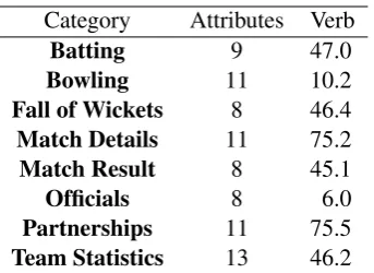
Table 1: Number of attributes per category with percent verbalised (Verb)

with this by enforcing a stronger structure – di-viding the information into eight of our own ‘cat-egories’, based roughly on the formatting of the webpages. These are outlined in Table 1.

The first three categories in the table are quite intuitive and implicit from the respective sections of the scorecard. There is additional information in a typical scorecard (not shown in Figure 1), which we must also categorise. The ‘Team Statis-tics’ category contains details about the ‘extras’3 scored by each team, as well as the number of points gained by the team towards that particular series4. We divide the remaining tag attributes as follows into three categories: ‘Officials’ – persons participating in the match, other than the teams (e.g. umpires, referees); ‘Match Details’ – infor-mation that would have been known before the match was played (e.g. venue, date, season); and ‘Match Result’ – data that could only be known once the match was over (e.g. final result, player of the match).

Finally we have an additional ‘Partnerships’5 category which is given explicitly on a separate webpage referenced from each scorecard, but is also implicit from information contained in the ‘Fall of Wickets’ and ‘Batting’ sections. We an-ticipate that this category will help us manage the issue of data sparsity. For instance, in our domain we could group partnerships (which could con-tain a multitude of player combinations and

there-3

Additional runs awarded to the batting team for specific actions executed by the bowling team. There are four types: No Ball, Wide, Bye, Leg Bye.

4_{Each cricket game is part of a specific ‘series’ of games.}

e.g. India would receive five points for their win within the NatWest series.

5_{A ‘partnership’ refers to a pair of players who bat}

to-gether, and usually comprises information such as the num-ber of runs scored between them, the numnum-ber of deliveries faced and so on.

fore distinct tags) with the various possible binary combinations of players together for shared learn-ing. We discuss this further in Section 8.3.

Within 5 of the categories described above, we are further able to divide the data into ‘groups’ -the Batting, Bowling, Fall of Wickets and Partner-ships categories refer to multiple players and thus have multiple rows. The Team Statistics category contains two groups, one for each team. The other categories merely form one-line tables.

4 Machine Learning

Our task is to establish which tag attributes (and hence tag values) should be included in the final match report, and is a multi-label classification problem. We chose to use BoosTexter (Schapire and Singer, 2000) as it has been shown to be an effective classifier (Yang, 1999), and it is one of the few text classification tools which directly sup-ports multi-label classification. This is also what B&L used.

Schapire and Singer’s BoosTexter (2000) uses ‘decision stumps’, or single level decision trees to classify its input data. The predicates of these stumps are defined, for text, by the presence or absence of a single term, and, for numerical at-tributes, whether the attribute exceeds a given threshold, decided dynamically.

4.1 Running BoosTexter

BoosTexter requires two input files to train a hy-pothesis, ‘Names’ and ‘Data’.

Names The Names file contains, for each pos-sible tag attribute,t, across all scorecards, the type of its corresponding tag value. These are contin-uousfor numbers and textfor normal text. From our 133 scorecards we extracted a total of 61,063 tag values, of which 82.2% were continuous, the remainder beingtext.

DataThe Data file contains, for each scorecard, a comma-delimited list of all tag values for a par-ticular scorecard, with a ‘?’ for unknown values, followed by a list of the verbalised tag attributes.

to the test scorecard, while|f|is a measure of the confidence the classifier has in its assertion.

4.2 Data Sparsity

The very nature of the data means that there are a large number of tag values which do not occur in every scorecard – the average scorecard con-tained 24 values, yet our ‘names’ file concon-tained 1193 possible tag attributes. A lot of this was due to partnership tag attributes which formed 43.6% of the ‘names’ entries. This large figure is because a large number of all possible binary combinations of players existed in the training data across both teams6. This implies we will be unable to train for a significant number of tag attributes as many spe-cific tag values occur very rarely. Indeed we found that of 158,669 entries, 97,666 (61.55%) were ‘un-known’.

5 Evaluation Baselines

It is not clear what constitutes a suitable baseline so we considered multiple options. The issue of ambiguous reference baselines is not specific to the cricket domain, as there is no standardized baseline approach across the prior literature. We employ ten-fold cross validation throughout.

5.1 Majority Baseline

B&L created a ‘majority baseline’ whereby they returned those categories (i.e., tables) which were verbalised more than half of the time in their aligned reports.

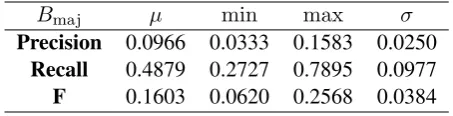
As explained in Section 3.2 we divided our tag attributes into 8 categories. We emulated B&L’s baseline method as follows: For each category, if any of the tag values within a particular ‘group’ was tagged as verbalised, we counted that as a ‘vote’ for that particular category. We then cal-culated the total number of ‘votes’ divided by the total number of ‘groups’ within each category. All categories which had a ratio of 50% or greater in this calculation were considered to be ‘major-ity categories’. Our baselineBmajthen consisted of all tag attributes forming part of those majority categories. As shown in Table 1 there were only two categories which exceeded the 50% threshold, ‘Match Details’ and ‘Partnerships’.

We can see that this baseline performs abysmally. The reason for this poor behaviour is

6_{93 of the possible2}P10

i=1i = 110 combinations

oc-curred.

Bmaj µ min max σ

Precision 0.0966 0.0333 0.1583 0.0250 Recall 0.4879 0.2727 0.7895 0.0977

F 0.1603 0.0620 0.2568 0.0384

Table 2: Majority Baseline,Bmaj

that since so many tag attributes contribute to the categories we are including far too many possibil-ities in our baseline.

5.2 Probabilistic Baseline

This baseline is based on the premise that those tag attributes which occur with highest frequency across the training data refer to those tag values which will often occur in a typical match report. To create our baseline set of tag attributes Bprob we extract theamost frequently verbalised tag at-tributes across all the training data whereais the average length of the verbalised tag attribute lists for each report/scorecard pair.

Bprob µ min max σ

Precision 0.5157 0.2174 0.7391 0.1010 Recall 0.5157 0.1389 0.7647 0.0990

F 0.5100 0.1695 0.6939 0.0852

Table 3: Probabilistic Baseline,Bprob

This baseline achieves a mean F score of 51%, however the tag attributes being returned are very inconsistent with a typical match report – they correspond in the majority to player names but not one refers to any other tag attributes relevant to those players. This renders the output mostly meaningless in terms of our aim to select content for an NLG system.

5.3 No-Player Probabilistic Baseline

with any and all corresponding player-name tag at-tributes7.

Bnops µ min max σ

Precision 0.4923 0.1765 0.6875 0.0922 Recall 0.3529 0.1111 0.5625 0.0842

F 0.4064 0.1538 0.5946 0.0767

Table 4: No-Player Probabilistic Baseline,Bnops

As can be seen from Table 4, this method suffers an absolute F-score drop of more than 10% from the previous method. However if we analyse the output more closely we can see that although the accuracy has dropped, the returned tag attributes are more thematically consistent with the training data. This is our preferred baseline.

6 Evaluation Paradigm

The main difficulty we encountered arose when we came to assessing the Precision and Recall fig-ures as we have yet to decide on what level we are considering the output of our system to be correct. We see three possibilities for the level:

Category We could simply count the ‘votes’ predicted on a per category basis (as described in sections 3.1 and 5.1), and evaluate categories based on the number of votes given for each. We would expect this to generate very good results as we are effectively overgrouping, once on a group basis (grouping together all attributes) and once on a category basis (unifying all groups within a cate-gory), but the output would be so general and triv-ial (effectively stating something to the effect that “a match report should contain information about batting, bowling and team statistics”) that it would be of no use in an NLG system.

GroupsHere we compare which ‘groups’ were verbalised within each category, and which were predicted to be verbalised (as we did for the Major-ity Baseline of Section 5.1). Our implicit grouping means that we do not have to necessarily return the correct statistic pertaining to a group since each group acts as a basket for the statistics contained within it, and is susceptible to ‘false positives’. This method is most similar to B&L’s.

TagsSince we are trying to establish whichtag attributes should be included rather than which

groups are likely to contain verbalised tag at-tributes, we could say that even the above method

7_{e.g., if}

team1 player4 Ris ina0then we would also in-cludeteam1 player4in our final set.

is too liberal in its definition of correctness. Thus we also evaluate our groups on the basis of their component parts, i.e., if a particular group of tag attributes is estimated to be verbalised by Boos-Texter, then we include all attributes from that group.

7 Initial Results

Our ‘categorized’ results are derived from present-ing BoosTexter with each individual category as described in Section 3.2, then merging the selected tag attributes together and evaluating based on the criteria described above. We then show BoosTex-ter’s performance ‘as is’, by running the program on the full output of our alignment stage with no categorization/grouping.

7.1 Categorized – Groups Level

Our ‘Categorized Groups’ results can be found in Figure 3 and Table 5. For each of our tests we vary the value ofT (the number of rounds) to see how it affects our accuracy.

Here we see we have a maximum F score of 0.7039 for T = 25. This is a very high result, performing far better than all our baselines, how-ever we feel the ‘basketing’ mentioned in Section 6 means that the results are not particularly in-structive – instead of specific ‘interesting’ tag at-tributes, we return a grouped list of tag atat-tributes, only some of which are likely to be ‘interesting’. Thus we decide to no longer pursue ‘grouping’ as a valid evaluation method, and evaluate all our methods at the ‘tag attribute’ level.

Best µ σ

Precision 0.7620 0.7473 0.0320 CG Recall 0.6795 0.6680 0.0322

F 0.7039 0.6897 0.0106

Table 5: Categorized Groups with Best value for T = 25.

7.2 Categorized – Tags Level

What is notable here is that, for all values of T which we ran our tests on (ranging from 1 to 3000), we obtained just one set of results for ‘Cat-egorized Tags’, displayed in Table 6.

0.4 0.5 0.6 0.7 0.8

1 10 100 1000

T

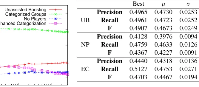
Unassisted Boosting Categorized Groups No Players Enhanced Categorization

Figure 3: All F scores Results

µ min max σ

Precision 0.0880 0.0496 0.1933 0.0223 Recall 0.7872 0.5417 1.0000 0.1096

F 0.1575 0.0924 0.3151 0.0361

Table 6: Categorized Tags Results

the very low Precision value. This method is ef-fectively a direct application of B&L’s method to our domain, however because of our strict accu-racy measurement, it does not perform particularly well. In fact it is even worse thanBmaj, our worst-performing baseline. We believe this is because the Majority Baseline is limited in the breadth of tags returned, whereas this method returns very large sets of over 200 tag attributes (due to the many contributing tag attributes of each category) while the average size of the training sets is 24.

Ideally we want to strike a balance between the improved granularity of the Categorized Tags evaluation (without the low accuracy) with the excellent performance of the Categorized Groups evaluation (without the too-broad basketing).

7.3 Unassisted Boosting

Our results are in Table 7 (row UB) and Figure 3. We can see F values are increasing on the whole, and that we have nearly reached our Probabilis-tic Baseline. Inspecting the contents of the sets returned by BoosTexter, we see they are slightly more in line with a typical training set, but still suf-fer from an over-emphasis on player names. We also believe the high number of rounds required for our best result (T = 2250) is caused by the sparsity issue described in Section 4.2.

Best µ σ

Precision 0.4965 0.4730 0.0253 UB Recall 0.4961 0.4723 0.0252

F 0.4907 0.4673 0.0249

Precision 0.4128 0.3976 0.0094 NP Recall 0.4759 0.4633 0.0126

F 0.4367 0.4227 0.0091

Precision 0.4440 0.4318 0.0136 EC Recall 0.5127 0.4753 0.0271

F 0.4703 0.4467 0.0194

Table 7: Unassisted Boosting (UB), No Players (NP) and Enhanced Categorization (EC). Best val-ues forT = 2250,250and20respectively.

8 No-Players & Enhanced Categorization

We now consider alternative, novel methods for improving our results.

8.1 Player Exclusion

We have thus far ignored coherency in our data – for example we want to make sure that player statistics will be accompanied by their correspond-ing player name.

One problem so far with our approach has been that we are effectively double-counting the play-ers. Our methods inspect which player names should appear at the same time as finding ap-propriate match statistics, whereas we believe we should instead be finding relevant statistics in the first instance, holding back player names, then in-cluding only those players to whom the statistics refer. Thus we restate our task in this way.

This is also sensible as in previous incarnations the learning algorithm had been learning from the literal strings of the player names. Although a player could be more likely to be named for vari-ous reasons, these reasons would not appear in the scorecard and we feel the strings are best ignored. Thus we decide to remove all player names from the machine learning input, reinstating only relevant ones once BoosTexter has selected its chosen tag attributes.

8.2 Player Exclusion Results

8.3 Enhanced Categorization

Our final method combines the ideas of Section 8.1 above with the benefits of categorization, and handles data sparsity issues.

The method is identical to that of Section 3.1, with two important exceptions: The first is that we reintroduce player names after the learning, as above. The second is that instead of just a bi-nary include/don’t-include decision for each tag attribute, we offer a list of verbalised tag attributes to the learner, butanonymising them with respect to the group in which they appear. This enables the learner to, given any group, predict which tag attributes should be returned, independent of the group in question. This means groups with often-empty tag values are able to leverage the informa-tion from groups with usually populated tag val-ues, hence solving our data-sparsity issues. For example, this will solve the issue, referenced in Section 4.2 of a lack of training data for particular player-combination partnerships.

Having held back the group to which the tag at-tributes belong, we reintroduce them enabling dis-covery of the original tag attribute. This offers the benefits of categorization, but with a finer-grained approach to the returned sets of tag attributes.

8.4 Enhanced Categorization Results

Our results are in Table 7 (row EC) and Figure 3. We achieved our best F score result of 0.4703 for a relatively low value ofT = 20, and we can clearly see that boosting establishes a reasonable ruleset after a small number of iterations – we be-lieve we have resolved the issue of data sparsity. The fact that this grouping has improved our re-sults compared to feeding the information in ‘flat’ (as in Section 7.3) emphasises that the construc-tion and make-up of the categories play a key role in defining performance.

9 Conclusions & Future Work

This paper has presented an exploration of various methods which could prove useful when select-ing content given a partially structured database of statistics and output text to emulate. We be-gan by acquiring the necessary domain data, in the form of scorecards and reports, and employed a six-step process to align scorecard statistics ver-balised in the reports. We next categorised our statistics based on the scorecard format. We es-tablished three baselines – one ‘unthinking’

proba-bilistic baseline, a ‘sensible’ probaproba-bilistic one, and another using categorization.

We found that unassisted boosting actually per-formed worse than our comparable probabilistic baseline, Bprob, but its output was marginally more in line with the typical training data. We explored how categorization affected our results, and showed that by grouping similar sets of tag attributes together we achieved a 7.4% improve-ment over the comparable baseline value, Bnops (Table 4). We further improved this technique in a novel way by sharing structural information be-tween learning instances, and by holding back cer-tain information from the learner. Our final best F-value marked a relative 15.7% increase onBnops.

There are multiple avenues still available for ex-ploration. One possibility would be to further in-vestigate the effects of categorization from Section 3.2, for example by varying the size and number of categories. We would also like to apply our meth-ods to another domain (e.g. rugby games) to es-tablish the relative generality of our approach.

Acknowledgments

This paper is based on Colin Kelly’s M.Phil. thesis, written towards his completion of the University of Cambridge Com-puter Laboratory’sComputer Speech, Text and Internet Tech-nologycourse. Grateful thanks go to the EPSRC for funding.

References

Regina Barzilay and Mirella Lapata. 2005. Collective Con-tent Selection for Concept-To-Text Generation. InHLT ‘05, pages 331–338. Association for Computational Lin-guistics.

Jose Coch. 1998. Multimeteo: multilingual production of weather forecasts.ELRA Newsletter, 3(2).

Cricinfo. 2007. Wisden Almanack.

http://cricinfo.com/wisdenalmanack. Retrieved 28 April 2007. Registration required.

Pablo A. Duboue and Kathleen R. McKeown. 2003. Statis-tical Acquisition of Content Selection Rules for Natural Language Generation.EMNLP ‘03, pages 121–128. Ehud Reiter and Robert Dale. 2000. Building Natural

Lan-guage Generation Systems. Cambridge University Press. Jacques Robin. 1995. Revision-based generation of

natu-ral language summaries providing historical background: corpus-based analysis, design, implementation and evalu-ation. Ph.D. thesis, Columbia University.

Robert E. Schapire and Yoram Singer. 2000. BoosTexter: A boosting-based system for text categorization.Machine Learning, 39(2/3):135–168.