Bandit Learning in Concave
N
-Person Games
Mario Bravo
Universidad de Santiago de Chile
Departamento de Matemática y Ciencia de la Computación mario.bravo.g@usach.cl
David Leslie
Lancaster University & PROWLER.io d.leslie@lancaster.ac.uk
Panayotis Mertikopoulos Univ. Grenoble Alpes, CNRS, Inria,
LIG 38000 Grenoble, France. panayotis.mertikopoulos@imag.fr
Abstract
This paper examines the long-run behavior of learning with bandit feedback in non-cooperative concave games. The bandit framework accounts for extremely low-information environments where the agents may not even know they are playing a game; as such, the agents’ most sensible choice in this setting would be to employ a no-regret learning algorithm. In general, this does not mean that the players’ behavior stabilizes in the long run: no-regret learning may lead to cycles, even with perfect gradient information. However, if a standard monotonicity condition is satisfied, our analysis shows that no-regret learning based on mirror descent with bandit feedback converges to Nash equilibrium with probability1. We also derive an upper bound for the convergence rate of the process that nearly matches the best attainable rate forsingle-agentbandit stochastic optimization.
1
Introduction
The bane of decision-making in an unknown environment isregret: noone wants to realize in hindsight that the decision policy they employed was strictly inferior to a plain policy prescribing the same action throughout. For obvious reasons, this issue becomes considerably more intricate when the decision-maker is subject to situational uncertainty and the “fog of war”: when the only information at the optimizer’s disposal is the reward obtained from a given action (the so-called “bandit” framework), is it even possible to design a no-regret policy? Especially in the context of online convex optimization (repeated decision problems with continuous action sets and convex costs), this problem becomes even more challenging because the decision-maker typically needs to infer gradient information from the observation of a single scalar. Nonetheless, despite this extra degree of difficulty, this question has been shown to admit a positive answer: regret minimizationis
possible, even with bandit feedback (Flaxman et al.,2005;Kleinberg,2004).
In this paper, we consider a multi-agent extension of this framework where, at each stagen= 1,2, . . ., of a repeated decision process, the reward of an agent is determined by the actions of all agents via a fixed mechanism:a non-cooperativeN-person game. In general, the agents – or players – might be completely oblivious to this mechanism, perhaps even ignoring its existence: for instance, when choosing how much to bid for a good in an online auction, an agent is typically unaware of who the other bidders are, what are their specific valuations, etc. Hence, lacking any knowledge about the game, it is only natural to assume that agents will at least seek to achieve a minimal worst-case guarantee and minimize their regret. As a result, a fundamental question that arises isa) whether the agents’ sequence of actions stabilizes to a rationally admissible state under no-regret learning; and
b) if it does, whether convergence is affected by the information available to the agents.
Related work. In finite games, no-regret learning guarantees that the players’ time-averaged, empirical frequency of play converges to the game’s set of coarse correlated equilibria (CCE), and the rate of this convergence isO(1/n)for(λ, µ)-smooth games (Foster et al.,2016;Syrgkanis et al., 2015). In general however, this set might contain highly subpar, rationally inadmissible strategies: for instance,Viossat and Zapechelnyuk(2013) provide examples of CCE that assign positive selection probabilityonlyto strictly dominated strategies. In the class of potential games,Cohen et al.(2017) recently showed that theactualsequence of play (i.e., the sequence of actions that determine the agents’ rewards at each stage) converges under no-regret learning, even with bandit feedback. Outside this class however, the players’ chosen actions may cycle in perpetuity, even in simple, two-player zero-sum games with full information (Mertikopoulos et al.,2018a,b); in fact, depending on the parameters of the players’ learning process, agents could even exhibit a fully unpredictable, aperiodic and chaotic behavior (Palaiopanos et al.,2017). As such, without further assumptions in place, no-regret learning in a multi-agent setting does not necessarily imply convergence to a unilaterally stable, equilibrium state.
In the broader context of games with continuous action sets (the focal point of this paper), the long-run behavior of no-regret learning is significantly more challenging to analyze. In the case of mixed-strategy learning,Perkins and Leslie(2014) andPerkins et al.(2017) showed that mixed-stratgy learning based on stochastic fictitious play converges to anε-perturbed Nash equilibrium in potential games (but may lead to as much asO(εn)regret in the process). More relevant for our purposes is the analysis ofNesterov(2009) who showed that the time-averaged sequence of play induced by a no-regret dual averaging (DA) process with noisy gradient feedback converges to Nash equilibrium in monotone games (a class which, in turn, contains all concave potential games).
The closest antecedent to our approach is the recent work ofMertikopoulos and Zhou(2018) who showed that theactualsequence of play generated by dual averaging converges to Nash equilibrium in the class of variationally stable games (which includes all monotone games). To do so, the authors first showed that a naturally associated continuous-time dynamical system converges, and then used the so-calledasymptotic pseudotrajectory(APT) framework ofBenaïm(1999) to translate this result to discrete time. Similar APT techniques were also used in a very recent preprint byBervoets et al.(2018) to establish the convergence of apayoff-based learning algorithm in two classes of one-dimensional concave games: games with strategic complements, and ordinal potential games with isolated equilibria. The algorithm ofBervoets et al.(2018) can be seen as a special case of mirror descent coupled with a two-point gradient estimation process, suggesting several interesting links with our paper.
Our contributions. In this paper, we drop all feedback assumptions and we focus on thebandit
framework where the only information at the players’ disposal is the payoffs they receive at each stage. As we discussed above, this lack of information complicates matters considerably because players must now estimate their payoff gradients from their observed rewards. What makes matters even worse is that an agent may introduce a significant bias in the (concurrent) estimation process of another, so traditional, multiple-point estimation techniques for derivative-free optimization cannot be applied (at least, not without significant communication overhead between players).
To do away with player coordination requirements, we focus on learning processes which could be sensibly deployed in a single-agent setting and we show that, in monotone games, the sequence of play induced by a wide class of no-regret learning policies converges to Nash equilibrium with probability1. Furthermore, by specializing to the class of strongly monotone games, we show that the rate of convergence isO(n−1/3), i.e., it is nearly optimal with respect to the attainableO(n−1/2)
rate for bandit,single-agentstochastic optimization with strongly convex and smooth objectives (Agarwal et al.,2010;Shamir,2013).
2
Problem setup and preliminaries
Concave games. Throughout this paper, we will focus on games with a finite number of players i∈ N ={1, . . . , N}and continuous action sets. During play, every playeri∈ N selects anaction
xifrom a compact convex subsetXiof adi-dimensional normed spaceVi; subsequently, based on each player’s individual objective and theaction profilex= (xi;x−i)≡(x1, . . . , xN)of all players’ actions, every player receives areward, and the process repeats. In more detail, writingX ≡Q
iXi for the game’saction space, we assume that each player’s reward is determined by an associated
payoff (orutility)functionui:X →R. Since players are not assumed to “know the game” (or even that they are involved in one) these payoff functions might be a priori unknown, especially with respect to the dependence on the actions of other players. Our only structural assumption foruiwill be thatui(xi;x−i)is concave inxifor allx−i∈ X−i≡Qj6=iXj,i∈ N.
With all this in hand, aconcave gamewill be a tupleG ≡ G(N,X, u)with players, action spaces and payoffs defined as above. Below, we briefly discuss some examples thereof:
Example 2.1(Cournot competition). In the standard Cournot oligopoly model, there is a finite set of
firmsindexed byi= 1, . . . , N, each supplying the market with a quantityxi∈[0, Ci]of some good (or service), up to the firm’s production capacityCi. By the law of supply and demand, the good is priced as a decreasing functionP(xtot)of the total amountxtot=P
N
i=1xisupplied to the market, typically following a linear model of the formP(xtot) =a−bxtotfor positive constantsa, b >0.
The utility of firmiis then given by
ui(xi;x−i) =xiP(xtot)−cixi, (2.1)
i.e., it comprises the total revenue from producingxiunits of the good in question minus the associated production cost (in the above,ci>0represents the marginal production cost of firmi).
Example 2.2(Resource allocation auctions). Consider a service provider with a number of splittable
resourcess ∈ S = {1, . . . , S} (bandwidth, server time, GPU cores, etc.). These resources can be leased to a set ofN bidders (players) who can place monetary bidsxis ≥0for the utilization of each resources ∈ S up to each player’s total budgetbi, i.e.,Ps∈Sxis ≤ bi. Once all bids are in, resources are allocated proportionally to each player’s bid, i.e., thei-th player getsρis = (qsxis)
(cs+Pj∈Nxjs)units of thes-th resource (whereqsdenotes the available units of said resource andcs≥0is the “entry barrier” for bidding on it). A simple model for the utility of playeri is then given by
ui(xi;x−i) =
X
s∈S
[giρis−xis], (2.2)
withgidenoting the marginal gain of playerifrom acquiring a unit slice of resources.
Nash equilibrium and monotone games. The most widely used solution concept for non-cooperative games is that of aNash equilibrium(NE), defined here as any action profilex∗∈ X that is resilient to unilateral deviations, viz.
ui(x∗i;x
∗
−i)≥ui(xi;x∗−i) for allxi∈ Xi,i∈ N. (NE)
By the classical existence theorem ofDebreu(1952), every concave game admits a Nash equilibrium. Moreover, thanks to the individual concavity of the game’s payoff functions, Nash equilibria can also be characterized via the first-order optimality condition
hvi(x∗), xi−xi∗i ≤0 for allxi∈ Xi, (2.3)
wherevi(x)denotes the individual payoff gradient of thei-th player, i.e.,
vi(x) =∇iui(xi;x−i), (2.4)
with∇idenoting differentiation with respect toxi.1In terms of regularity, it will be convenient to assume that eachviis Lipschitz continuous; to streamline our presentation, this will be our standing assumption in what follows.
1
We adopt here the standard convention of treatingvi(x)as an element of the dual spaceYi≡ Vi∗ofVi,
Starting with the seminal work ofRosen(1965), much of the literature on continuous games and their applications has focused on games that satisfy a condition known asdiagonal strict concavity(DSC). In its simplest form, this condition posits that there exist positive constantsλi>0such that
X
i∈N
λihvi(x0)−vi(x), x0i−xii<0 for allx, x0 ∈ X,x6=x0. (DSC)
Owing to the formal similarity between (DSC) and the various operator monotonicity conditions in optimization (see e.g.,Bauschke and Combettes,2017), games that satisfy (DSC) are commonly referred to as (strictly)monotone. As was shown byRosen(1965, Theorem 2), monotone games admit a unique Nash equilibriumx∗ ∈ X, which, in view of (DSC) and (NE), is also the unique solution of the (weighted) variational inequality
X
i∈N
λihvi(x), xi−x∗ii<0 for allx6=x∗. (VI)
This property of Nash equilibria of monotone games will play a crucial role in our analysis and we will use it freely in the rest of our paper.
In terms of applications, monotonicity gives rise to a very rich class of games. As we show in the paper’s supplement,Examples 2.1and2.2both satisfy diagonal strict concavity (with a nontrivial choice of weights for the latter), as do atomic splittable congestion games in networks with parallel links (Orda et al.,1993;Sorin and Wan,2016), multi-user covariance matrix optimization problems in multiple-input and multiple-output (MIMO) systems (Mertikopoulos et al.,2017), and many other problems where online decision-making is the norm. Namely, the class of monotone games contains all strictly convex-concave zero-sum games and all games that admit a (strictly) concavepotential, i.e., a functionf:X →Rsuch thatvi(x) =∇if(x)for allx∈ X,i∈ N. In view of all this (and unless explicitly stated otherwise), we will focus throughout on monotone games; for completeness, we also include in the supplement a straightforward second-order test for monotonicity.
3
Regularized no-regret learning
We now turn to the learning methods that players could employ to increase their individual rewards in an online manner. Building onZinkevich’s (2003) online gradient descent policy, the most widely used algorithmic schemes for no-regret learning in the context of online convex optimization invariably revolve around the idea ofregularization. To name but the most well-known paradigms, “following the regularized leader” (FTRL) explicitly relies on best-responding to a regularized aggregate of the reward functions revealed up to a given stage, while online mirror descent (OMD) and its variants use a linear surrogate thereof. All these no-regret policies fall under the general umbrella of “regularized learning” and their origins can be traced back to the seminalmirror descent(MD) algorithm of Nemirovski and Yudin(1983).2
The basic idea of mirror descent is to generate a new feasible pointx+by taking a so-called “mirror
step” from a starting pointxalong the direction of an “approximate gradient” vectory(which we treat here as an element of the dual spaceY ≡Q
iYiofV ≡QiVi).3 To do so, lethi:Xi→Rbe a continuous andKi-strongly convexdistance-generating(orregularizer) function, i.e.,
hi(txi+ (1−t)x0i)≤thi(xi) + (1−t)hi(x0i)−12Kit(1−t)kx
0
i−xik2, (3.1)
for allxi, x0i ∈ Xi and allt ∈ [0,1]. In terms of smoothness (and in a slight abuse of notation) we also assume that the subdifferential of hi admits a continuous selection, i.e., a continuous function∇hi: dom∂hi → Yisuch that∇hi(xi)∈∂hi(xi)for allxi ∈dom∂hi.4 Then, letting
2
In a utility maximization setting, mirror descent should be called mirrorascentbecause players seek to maximizetheir rewards (as opposed tominimizingtheir losses). Nonetheless, we keep the term “descent” throughout because, despite the role reversal, it is the standard name associated with the method.
3
For concreteness (and in a slight abuse of notation), we assume in what follows thatVis equipped with the product normkxk2
=P
ikxik 2
andYwith the dual normkyk∗= max{hy, xi:kxk ≤1}. 4
Recall here that the subdifferential ofhiatxi∈ Xiis defined as∂hi(xi)≡ {yi∈ Yi:hi(x0i)≥hi(xi) +
hyi, x0i−xiifor allx0i∈ Vi},with the standard convention thathi(xi) = +∞ifxi∈ Vi\ Xi. By standard
h(x) = P
ihi(xi)forx ∈ X (sohis strongly convex with modulusK = miniKi), we get a
pseudo-distanceonXvia the relation
D(p, x) =h(p)−h(x)− h∇h(x), p−xi, (3.2)
for allp∈ X,x∈dom∂h.
This pseudo-distance is known as theBregman divergenceand we haveD(p, x)≥0with equality if and only ifx = p; on the other hand,D may fail to be symmetric and/or satisfy the triangle inequality so, in general, it is not a bona fide distance function onX. Nevertheless, we also have D(p, x)≥ 1
2Kkx−pk
2(see the paper’s supplement), so the convergence of a sequenceX
ntop can be checked by showing thatD(p, Xn) → 0. For technical reasons, it will be convenient to also assume the converse, i.e., thatD(p, Xn)→0whenXn→p. This condition is known in the literature as “Bregman reciprocity” (Chen and Teboulle,1993), and it will be our blanket assumption in what follows (note that it is trivially satisfied byExamples 3.1and3.2below).
Now, as with true Euclidean distances,D(p, x)induces aprox-mappinggiven by
Px(y) = arg min x0∈X
{hy, x−x0i+D(x0, x)} (3.3)
for allx∈dom∂hand ally∈ Y. Just like its Euclidean counterpart below, the prox-mapping (3.3) starts with a pointx∈dom∂hand steps along the dual (gradient-like) vectory∈ Yto produce a new feasible pointx+ =Px(y). Standard examples of this process are:
Example 3.1(Euclidean projections). Leth(x) = 12kxk2
2denote the Euclidean squared norm. Then,
the induced prox-mapping is
Px(y) = Π(x+y), (3.4)
withΠ(x) = arg minx0∈Xkx0−xk2denoting the standard Euclidean projection ontoX. Hence, the update rulex+=Px(y)boils down to a “vanilla”, Euclidean projection step alongy.
Example 3.2(Entropic regularization and multiplicative weights). Suppressing the player index for simplicity, let X be ad-dimensional simplex and consider the entropic regularizerh(x) =
Pd
j=1xjlogxj. The induced pseudo-distance is the so-calledKullback–Leibler(KL) divergence DKL(p, x) =Pdj=1pjlog(pj/xj),which gives rise to the prox-mapping
Px(y) =
(xjexp(yj))dj=1
Pd
j=1xjexp(yj)
(3.5)
for allx∈ X◦,y∈ Y. The update rulex+=P
x(y)is widely known as themultiplicative weights (MW) algorithm and plays a central role for learning in multi-armed bandit problems and finite games (Arora et al.,2012;Auer et al.,1995;Freund and Schapire,1999).
With all this in hand, the multi-agentmirror descent(MD) algorithm is given by the recursion
Xn+1=PXn(γnˆvn), (MD)
whereγnis a variable step-size sequence andvˆn = (ˆvi,n)i∈N is a generic feedback sequence of
estimated gradients. In the next section, we detail how this sequence is generated with first- or zeroth-order (bandit) feedback.
4
First-order vs. bandit feedback
4.1 First-order feedback.
A common assumption in the literature is that players are able to obtain gradient information by querying afirst-order oracle(Nesterov,2004). i.e., a “black-box” feedback mechanism that outputs an estimatevˆiof the individual payoff gradientvi(x)of thei-th player at the current action profile x = (xi;x−i) ∈ X. This estimate could be eitherperfect, givingvˆi = vi(x)for alli ∈ N, or
Having access to a perfect oracle is usually a tall order, either because payoff gradients are difficult to compute directly (especially without global knowledge), because they involve an expectation over a possibly unknown probability law, or for any other number of reasons. It is therefore more common to assume that each player has access to astochastic oraclewhich, when called against a sequence of actionsXn ∈ X, produces a sequence of gradient estimatesˆvn = (vi,n)i∈N that satisfies the
following statistical assumptions:
a)Unbiasedness: E[ˆvn| Fn] =v(Xn).
b)Finite mean square: E[kˆvnk2∗| Fn]≤V2 for some finiteV ≥0.
(4.1)
In terms of measurability, the expectation in (4.1) is conditioned on the historyFnofXnup to stage n; in particular, sincevˆnis generated randomly fromXn, it is notFn-measurable (and hence not adapted). To make this more transparent, we will writevˆn =v(Xn) +Un+1whereUnis an adapted martingale difference sequence withE[kUn+1k2∗| Fn]≤σ2for some finiteσ≥0.
4.2 Bandit feedback.
Now, if players don’t have access to a first-order oracle – the so-called banditor payoff-based
framework – they will need to derive an individual gradient estimate from the only information at their disposal: the actual payoffs they receive at each stage. When a function can be queried at multiple points (as few as two in practice), there are efficient ways to estimate its gradient via directional sampling techniques as inAgarwal et al.(2010). In a game-theoretic setting however, multiple-point estimation techniques do not apply because, in general, a player’s payoff function depends on the actions ofallplayers. Thus, when a player attempts to get a second query of their payoff function, this function may have already changed due to the query of another player – i.e., instead of samplingui(·;x−i), thei-th player would be samplingui(·;x0−i)for somex0−i6=x−i.
FollowingSpall(1997) andFlaxman et al.(2005), we posit instead that players rely on a simultaneous perturbation stochastic approximation (SPSA) approach that allows them to estimate their individual payoff gradientsvibased off asinglefunction evaluation. In detail, the key steps of this one-shot estimation process for each playeri∈ N are:
0. Fix aquery radiusδ >0.5
1. Pick apivot pointxi∈ Xiwhere playeriseeks to estimate their payoff gradient.
2. Draw a vectorzifrom the unit sphereSi≡SdiofV
i≡Rdiand playxˆ
i=xi+δzi.6 3. Receiveuˆi=ui(ˆxi; ˆx−i)and set
ˆ vi=
di
δuˆizi. (4.2)
By adapting a standard argument based on Stokes’ theorem (detailed in the supplement), it can be shown thatˆviis an unbiased estimator of the individual gradient of theδ-smoothed payoff function
uδi(x) = 1
vol(δBi)Qj6=ivol(δSj)
Z
δBi
Z
Q
j6=iδSj
ui(xi+wi;x−i+z−i)dz1· · ·dwi· · ·dzN (4.3)
withBi≡Bdidenoting the unit ball ofV
i. The Lipschitz continuity ofviguarantees thatk∇iui− ∇iuδik∞ = O(δ), so this estimate becomes more and more accurate asδ → 0+. On the other
hand, the second moment ofvˆigrows asO(1/δ2),implying in turn that the variability ofvˆigrows unbounded asδ → 0+. This manifestation of the bias-variance dilemma plays a crucial role in
designing no-regret policies with bandit feedback (Flaxman et al.,2005;Kleinberg,2004), soδmust be chosen with care.
Before dealing with this choice though, it is important to highlight two feasibility issues that arise with the single-shot SPSA estimate (4.2). The first has to do with the fact that the perturbation directionziis chosen from the unit sphereSiso it may fail to be tangent toXi, even whenxi is interior. To iron out this wrinkle, it suffices to samplezifrom the intersection ofSiwith the affine
5
For simplicity, we takeδequal for all players; the extension to player-specificδis straightforward, so we omit it.
6
hull ofXiinVi; on that account (and without loss of generality), we will simply assume in what follows that eachXiis aconvex bodyofVi, i.e., it has nonempty topological interior.
The second feasibility issue concerns the size of the perturbation step: even ifziis a feasible direction of motion, the query pointxˆi=xi+δzimay be unfeasible ifxiis too close to the boundary ofXi. For this reason, we will introduce a “safety net” in the spirit ofAgarwal et al.(2010), and we will constrain the set of possible pivot pointsxito lie within a suitably shrunk zone ofX.
In detail, let Bri(pi)be anri-ball centered atpi ∈ Xi so thatBri(pi) ⊆ Xi. Then, instead of perturbingxibyzi, we consider thefeasibility adjustment
wi=zi−ri−1(xi−pi), (4.4)
and each player playsxˆi=xi+δwiinstead ofxi+δzi. In other words, this adjustment moves each pivot toxδi =xi−r−i 1δ(xi−pi), i.e.,O(δ)-closer to the interior base pointpi, and then perturbsxδi byδzi. Feasibility of the query point is then ensured by noting that
ˆ
xi=xδi +δzi= (1−ri−1δ)xi+ri−1δ(pi+rizi), (4.5)
soxˆi∈ Xiifδ/ri <1(sincepi+rizi ∈Bri(pi)⊆ Xi).
The difference between this estimator and the oracle framework we discussed above is twofold. First, each player’srealizedaction isxˆi =xi+δwi, notxi, so there is a disparity between the point at which payoffs are queried and the action profile where the oracle is called. Second, the resulting estimatorˆvis not unbiased, so the statistical assumptions (4.1) for a stochastic oracle do not hold. In particular, given the feasibility adjustment (4.4), the estimate (4.2) withxˆgiven by (4.5) satisfies
E[ˆvi] =∇iuδi(x δ i;x
δ
−i), (4.6)
so there aretwosources of systematic error: anO(δ)perturbation in the function, and anO(δ) perturbation of each player’s pivot point fromxitoxδi. Hence, to capture both sources of bias and separate them from the random noise, we will write
ˆ
vi =vi(x) +Ui+bi (4.7)
whereUi= ˆvi−E[ˆvi]andbi=∇iuδi(x δ)− ∇
iui(x). We are thus led to the following manifestation of the bias-variance dilemma: the bias termbin (4.7) isO(δ), but the second moment of the noise termU isO(1/δ2); as such, an increase in accuracy (small bias) would result in a commensurate
loss of precision (large noise variance). Balancing these two factors will be a key component of our analysis in the next section.
5
Convergence analysis and results
Combining the learning framework ofSection 3with the single-shot gradient estimation machinery ofSection 4, we obtain the following variant of (MD) with payoff-based,bandit feedback:
ˆ
Xn=Xn+δnWn, Xn+1=PXn(γnvˆn).
(MD-b)
In the above, the perturbationsWnand the estimatesˆvnare given respectively by (4.4) and (4.2), i.e.,
Wi,n=Zi,n−r−i 1(Xi,n−pi) vˆi,n= (di/δn)ui( ˆXn)Zi,n (5.1)
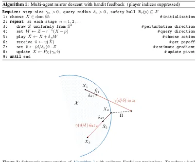
andZi,nis drawn independently and uniformly across players at each stagen(see alsoAlgorithm 1 for a pseudocode implementation andFig. 1for a schematic representation).
In the rest of this paper, our goal will be to determine the equilibrium convergence properties of this scheme in concaveN-person games. Our first asymptotic result below shows that, under (MD-b), the players’ learning process converges to Nash equilibrium in monotone games:
Theorem 5.1. Suppose that the players of a monotone gameG ≡ G(N,X, u)follow(MD-b)with step-sizeγnand query radiusδnsuch that
lim
n→∞γn = limn→∞δn= 0, ∞
X
n=1
γn=∞,
∞
X
n=1
γnδn<∞, and
∞
X
n=1
γ2
n δ2
n
<∞. (5.2)
Algorithm 1:Multi-agent mirror descent with bandit feedback (player indices suppressed)
Require: step-size γn>0, query radius δn>0, safety ball Br(p)⊆ X
1: choose X ∈dom∂h # initialization
2: repeat at each stage n= 1,2, . . .
3: draw Z uniformly from Sd # perturbation direction
4: set W ←Z−r−1(X−p) # query direction
5: play Xˆ ←X+δnW # choose action
6: receive ˆu←u( ˆX) # get payoff
7: set vˆ←(d/δn)ˆu·Z # estimate gradient
8: update X ←PX(γnˆv) # update pivot
9: until end
X X1
.
ˆ
X1
.
γ(d/δ) ˆu1z1
δz1
. X2
Π
.
ˆ
X2
. X3
γ(d/δ) ˆu2z2
[image:8.612.103.506.70.403.2]δz2
Figure 1: Schematic representation ofAlgorithm 1with ordinary, Euclidean projections. To reduce visual clutter, we did not include the feasibility adjustmentr−1(x−p)in the action selection stepXn7→Xˆn.
Even though the setting is different, the conditions (5.2) for the tuning of the algorithm’s parameters are akin to those encountered in Kiefer–Wolfowitz stochastic approximation schemes and serve a similar purpose. First, the conditionslimn→∞γn = 0andP∞n=1γn =∞respectively mitigate the method’s inherent randomness and ensure a horizon of sufficient length. The requirement limn→∞δn= 0is also straightforward to explain: as players accrue more information, they need to decrease the sampling bias in order to have any hope of converging. However, as we discussed in Section 4, decreasingδalso increases the variance of the players’ gradient estimates, which might grow to infinity asδ→0. The crucial observation here is that new gradients enter the algorithm with a weight ofγnso the aggregate bias afternstages is of the order ofO(Pnk=1γkδk)and its variance is O(Pn
k=1γ 2
k/δ
2
k). If these error terms can be controlled, there is an underlying drift that emerges over time and which steers the process to equilibrium. We make this precise in the supplement by using a suitably adjusted variant of the Bregman divergence as a quasi-Féjér energy function for (MD-b) and relying on a series of (sub)martingale convergence arguments to establish the convergence ofXˆn (first as a subsequence, then with probability1).
Of course, sinceTheorem 5.1is asymptotic in nature, it is not clear how to chooseγnandδnso as to optimize the method’s convergence rate. Heuristically, if we take schedules of the formγn=γ/np andδn=δ/nqwithγ, δ >0and0< p, q≤1, the only conditions imposed by (5.2) arep+q >1 andp−q >1/2. However, as we discussed above, the aggregate bias in the algorithm afternstages isO(Pn
k=1γnδn) =O(1/np+q−1)and its variance isO(P n k=1γ
2
k/δ
2
k) =O(1/n
2p−2q−1): if the
We show below that this bound is indeed attainable for games that arestrongly monotone, i.e., they satisfy the following stronger variant of diagonal strict concavity:
X
i∈N
λihvi(x0)−vi(x), x0i−xii ≤ − β 2kx−x
0k2 (β-DSC)
for someλi, β >0and for allx, x0∈ X. Focusing for expository reasons on the most widely used, Euclidean incarnation of the method (Example 3.1), we have:
Theorem 5.2. Letx∗be the(necessarily unique)Nash equilibrium of aβ-strongly monotone game.
If the players follow(MD-b)with Euclidean projections and parametersγn=γ/nandδn=δ/n1/3
withγ >1/(3β)andδ >0, we have
E[kXˆn−x∗k2] =O(n−1/3). (5.3)
Theorem 5.2is our main finite-time analysis result, so some remarks are in order. First, the step-size scheduleγn ∝ 1/nis not required to obtain anO(n−1/3)convergence rate: as we show in the paper’s supplement, more general schedules of the formγn∝1/npandδn∝1/nq withp >3/4 andq=p/3 > 1/4, still guarantee anO(n−1/3)rate of convergence for (MD-b). To put things
in perspective, we also show in the supplement that if (MD) is run with first-order oracle feedback satisfying the statistical assumptions (4.1), the rate of convergence becomesO(1/n). Viewed in this light, the price for not having access to gradient information is no higher thanO(n−2/3)in terms of
the players’ equilibration rate.
Finally, it is also worth comparing the bound (5.3) to the attainable rates for stochastic convex optimization (the single-player case). For problems with objectives that are both strongly convex and smooth,Agarwal et al.(2010) attained anO(n−1/2)convergence rate with bandit feedback, which
Shamir(2013) showed is unimprovable. Thus, in the single-player case, the bound (5.3) is off by n1/6and coincides with the bound ofAgarwal et al.(2010) for strongly convex functions that are not
necessarily smooth. One reason for this gap is that theΘ(n−1/2)bound ofShamir(2013) concerns
the smoothed-out time averageX¯n=n−1P n
k=1Xk, while our analysis concerns the sequence of
realized actionsXˆn. This difference is semantically significant: In optimization, the query sequence is just a means to an end, and only the algorithm’s output matters (i.e.,X¯n). In a game-theoretic setting however, it is the players’realizedactions that determine their rewards at each stage, so the figure of merit is the actual sequence of playXˆn. This sequence is more difficult to control, so this disparity is, perhaps, not too surprising; nevertheless, we believe that this gap can be closed by using a more sophisticated single-shot estimate, e.g., as inGhadimi and Lan(2013). We defer this analysis to the future.
6
Concluding remarks
The most sensible choice for agents who are oblivious to the presence of each other (or who are simply conservative), is to deploy a no-regret learning algorithm. With this in mind, we studied the long-run behavior of individual regularized no-regret learning policies and we showed that, in monotone games, play converges to equilibrium with probability1, and the rate of convergence almost matches the optimal rates ofsingle-agent, stochastic convex optimization. Nevertheless, several questions remain open: whether there is an intrinsic information-theoretic obstacle to bridging this gap; whether our convergence rate estimates hold with high probability (and not just in expectation); and whether our analysis extends to a fully decentralized setting where the players’ updates need not be synchronous. We intend to address these questions in future work.
Acknowledgments
References
Agarwal, Alekh, O. Dekel, L. Xiao. 2010. Optimal algorithms for online convex optimization with multi-point bandit feedback.COLT ’10: Proceedings of the 23rd Annual Conference on Learning Theory.
Arora, Sanjeev, Elad Hazan, Satyen Kale. 2012. The multiplicative weights update method: A meta-algorithm and applications.Theory of Computing8(1) 121–164.
Auer, Peter, Nicolò Cesa-Bianchi, Yoav Freund, Robert E. Schapire. 1995. Gambling in a rigged casino: The adversarial multi-armed bandit problem.Proceedings of the 36th Annual Symposium on Foundations of Computer Science.
Bauschke, Heinz H., Patrick L. Combettes. 2017.Convex Analysis and Monotone Operator Theory in Hilbert Spaces. 2nd ed. Springer, New York, NY, USA.
Benaïm, Michel. 1999. Dynamics of stochastic approximation algorithms. Jacques Azéma, Michel Émery, Michel Ledoux, Marc Yor, eds.,Séminaire de Probabilités XXXIII,Lecture Notes in Mathematics, vol. 1709. Springer Berlin Heidelberg, 1–68.
Bervoets, Sebastian, Mario Bravo, Mathieu Faure. 2018. Learning with minimal information in continuous games.https://arxiv.org/abs/1806.11506.
Chen, Gong, Marc Teboulle. 1993. Convergence analysis of a proximal-like minimization algorithm using Bregman functions.SIAM Journal on Optimization3(3) 538–543.
Cohen, Johanne, Amélie Héliou, Panayotis Mertikopoulos. 2017. Learning with bandit feedback in potential games.NIPS ’17: Proceedings of the 31st International Conference on Neural Information Processing Systems.
Debreu, Gerard. 1952. A social equilibrium existence theorem.Proceedings of the National Academy of Sciences of the USA38(10) 886–893.
Flaxman, Abraham D., Adam Tauman Kalai, H. Brendan McMahan. 2005. Online convex optimization in the bandit setting: gradient descent without a gradient. SODA ’05: Proceedings of the 16th annual ACM-SIAM Symposium on Discrete Algorithms. 385–394.
Foster, Dylan J., Thodoris Lykouris, Kathrik Sridharan, Éva Tardos. 2016. Learning in games: Robustness of fast convergence.NIPS ’16: Proceedings of the 30th International Conference on Neural Information Processing Systems. 4727–4735.
Freund, Yoav, Robert E. Schapire. 1999. Adaptive game playing using multiplicative weights. Games and Economic Behavior2979–103.
Ghadimi, Saeed, Guanghui Lan. 2013. Stochastic first- and zeroth-order methods for nonconvex stochastic programming.SIAM Journal on Optimization23(4) 2341–2368.
Kleinberg, Robert D. 2004. Nearly tight bounds for the continuum-armed bandit problem.NIPS’ 04: Proceedings of the 18th Annual Conference on Neural Information Processing Systems.
Mertikopoulos, Panayotis, E. Veronica Belmega, Romain Negrel, Luca Sanguinetti. 2017. Distributed stochastic optimization via matrix exponential learning.IEEE Trans. Signal Process.65(9) 2277–2290.
Mertikopoulos, Panayotis, Bruno Lecouat, Houssam Zenati, Chuan-Sheng Foo, Vijay Chandrasekhar, Georgios Piliouras. 2018a. Optimistic mirror descent in saddle-point problems: Going the extra (gradient) mile.
https://arxiv.org/abs/1807.02629.
Mertikopoulos, Panayotis, Christos H. Papadimitriou, Georgios Piliouras. 2018b. Cycles in adversarial reg-ularized learning. SODA ’18: Proceedings of the 29th annual ACM-SIAM Symposium on Discrete Algorithms.
Mertikopoulos, Panayotis, Zhengyuan Zhou. 2018. Learning in games with continuous action sets and unknown payoff functions.Mathematical Programming.
Nemirovski, Arkadi Semen, David Berkovich Yudin. 1983. Problem Complexity and Method Efficiency in Optimization. Wiley, New York, NY.
Nesterov, Yurii. 2004. Introductory Lectures on Convex Optimization: A Basic Course. No. 87 in Applied Optimization, Kluwer Academic Publishers.
Nesterov, Yurii. 2009. Primal-dual subgradient methods for convex problems. Mathematical Programming
120(1) 221–259.
Orda, Ariel, Raphael Rom, Nahum Shimkin. 1993. Competitive routing in multi-user communication networks. IEEE/ACM Trans. Netw.1(5) 614–627.
Palaiopanos, Gerasimos, Ioannis Panageas, Georgios Piliouras. 2017. Multiplicative weights update with constant step-size in congestion games: Convergence, limit cycles and chaos.NIPS ’17: Proceedings of the 31st International Conference on Neural Information Processing Systems.
Perkins, Steven, Panayotis Mertikopoulos, David S. Leslie. 2017. Mixed-strategy learning with continuous action sets.IEEE Trans. Autom. Control62(1) 379–384.
Rosen, J. B. 1965. Existence and uniqueness of equilibrium points for concaveN-person games.Econometrica
33(3) 520–534.
Shamir, Ohad. 2013. On the complexity of bandit and derivative-free stochastic convex optimization.COLT ’13: Proceedings of the 26th Annual Conference on Learning Theory.
Sorin, Sylvain, Cheng Wan. 2016. Finite composite games: Equilibria and dynamics.Journal of Dynamics and Games3(1) 101–120.
Spall, James C. 1997. A one-measurement form of simultaneous perturbation stochastic approximation. Automatica33(1) 109–112.
Syrgkanis, Vasilis, Alekh Agarwal, Haipeng Luo, Robert E. Schapire. 2015. Fast convergence of regularized learning in games.NIPS ’15: Proceedings of the 29th International Conference on Neural Information Processing Systems. 2989–2997.
Viossat, Yannick, Andriy Zapechelnyuk. 2013. No-regret dynamics and fictitious play.Journal of Economic Theory148(2) 825–842.