Empirical Fuzzy Sets
Plamen P. Angelov1,2 and Xiaowei Gu 1*
1School of Computing and Communications, Lancaster University, Lancaster, LA1 4WA, UK 2Honorary Professor, Technical University of Sofia, boulevard Kliment Ohridski 8, Sofia, 1000, Bulgaria
e-mail: {p.angelov, x.gu3}@lancaster.ac.uk
Abstract
series of new algorithms such as εF classifiers, εF predictors, εF controllers, etc. This is left for the future research.
Keywords—membership functions, AnYa type fuzzy rule-based systems, empirical data analytics, naïve empirical fuzzy rule-based classifier, non-parametric.
1. Introduction
Fuzzy sets (FSs) theory and the fuzzy rule-based (FRB) systems have been defined over 50 years ago in the seminal paper by Professor Lotfi Zadeh [1] and now matured [2]. Since mid-1970s (Mamdani or Zadeh-Mamdani) [3] and since mid-1980s (Takagi-Sugeno) [4] FRB systems started to be developed and are now widely applied. Although, there are other types of fuzzy systems (relational [5], etc.), one particular type that was introduced recently by Angelov and Yager [6] called AnYa deserves a special attention. Both Mamdani and Takagi-Sugeno type of FRB share the exact same antecedent (IF) part and only (although significantly) differ by the consequent (THEN) part. AnYa type FRB, however, has a quite different antecedent (IF) part.
The main issue in the design of the FSs and FRB systems is how to define the MFs by which they are defined in first place. The traditional way of designing FSs, the subjective approach, has its own very strong rationale in the two-way process of: i) formalizing expert knowledge and representing it in a mathematical form through the membership functions (MFs), and ii) representing and extracting from data human-intelligible and understandable, transparent linguistic information in the form of IF …THEN… rules. In 1990s, in addition to the traditional subjective way of designing FSs, the so-called data driven design method started to be popular and was developed. Nonetheless, it is practically very difficult and controversial to define MFs both form experts and from data. This is also related to the more general issue of assumptions made and handcrafting that machine learning (including statistical methods) are facing and is now hotly researched.
membership values or parameters, but only (optionally) the labels/names of the linguistic terms, classes (if any)). For example, if we choose a car, we can simply say which one we like (or possibly how much), but we do not need to define each feature (price, max speed, etc.) or specify why. Moreover, with the proposed εFSs and εFRB systems, one can tackle heterogeneous data and combine categorical (e.g. gender, occupation, number of doors) with continuous and/or discrete variables like price, max speed, size, etc. Further, in this paper, we will demonstrate how, on the basis of εFSs and εFRB systems, one can build empirical fuzzy classifiers (εF Classifiers), predictors (εF Predictors), controllers (εF Controllers), etc. Moreover, these can be evolving, not just fixed structure. This will allow studying the dynamic changes in human preferences as well as building more efficient recommendation systems where the only necessary input form the users is the preference (“likes” or “retweets” or “clicks”).
(a) Traditional subjective approach (b) Traditional objective approach
(c) The proposed subjective approach (d) The proposed objective approach Fig.1. The flowcharts of the traditional approaches and the proposed approaches for system identification
2. Theoretical Basis
In this section, we will recall the theoretical basis needed for the proposed approach.
2.1. Fuzzy Sets and Fuzzy Rule-Based Systems
In this subsection, we will compare the Mamdani type [3], Takagi-Sugeno type [4] and AnYa type FRB systems [6]. To begin with, let us start with an illustrative example.
If we want to build a Mamdani type or Takagi-Sugeno type FRB system to divide hundreds of domestic dogs into three groups (“Small”, “Medium” and “Large”) based on their size in terms of length and weight, the following parameters are needed to be defined in order to build the antecedent (IF) parts of the fuzzy rules (FRs) [9]:
i) the types of MFs, i.e. triangular type, Gaussian type, bell type, etc. ii) linguistic terms for each FR;
iii) the area of influence for each FR, i.e. hyper-rectangle, -sphere, -ellipsoid (this is closely linked to the types of distance metric used);
iv) the prototypes for the FSs; v) the parameters for the MFs.
To classify the dogs into three groups, we firstly build three FRs expressed linguistically as follows:
1
Rule: IF
Length is Short AND
Weight isLight
THEN
Size isSmall
2
3
Rule : IF
Length isLong AND
Weight isHigh
THEN
Size isLarge
Based on the data measured from the 600 domestic dogs (the distribution of the data samples is shown in Fig. 2, the data is synthetic), for the linguistic variable “Length”, we might interpret “Short” as “around 20 cm”, “Medium” as “around 37 cm” and “Long” as “around 54 cm”. For the linguistic variable “Weight”, “Light” could be interpreted as “around 15 kg”, “Medium” as “around 32 kg” and “High” as “around 48 cm”. After we select the type of MFs (for example, triangular and Gaussian) and decide other parameters, finally we obtain the FRB systems as depicted in Fig.3.
(a) Distribution (b) Frequency Fig.2. Distribution of the sizes of 600 domestic dogs
(a) Triangular type MF (b) Gaussian type MF
Fig.3. Examples of Mamdani type and Takagi-Sugeno type FRB systems (the black asterisks are the prototypes) From the above example, one can see the following issues during the process:
i) Defining a MF requires many ad hoc decisions;
In addition, the so-called “curse of dimensionality” may result from handcrafting traditional FRB systems for high dimensional problems because of the exponential growth of the number of FSs required.
Alternatively, to design an AnYa type FRB system [6] with the same prototypes as being used in the previous example, one can easily form three data clouds and, based on them, derive three AnYa type FRs as follows. The visualization of the three data clouds, which are also the areas of influence of the three FRs, is provided in Fig.4.
1
Rule: IF
Length, Weight ~ 20
cm, 15kg
THEN
Size is Small
2
Rule : IF
Length, Weight ~ 37
cm, 32kg
THEN
Size is Medium
3
Rule : IF
Length, Weight ~ 54
cm, 48kg
THEN
Size is Large
Fig.4. AnYa type FRB system
As one can see, the AnYa type FRB system [6] simplifies the process of designing MFs and FRs. They are uniquely defined by vectors representing the focal points of the non-parametric, shape-free data clouds consisting of data samples associated with the nearest focal points resembling Voronoi tessellation [10]. The data clouds are then used as the antecedent (IF) part of each AnYa type FR. This significantly reduces the efforts of human experts and, at the same time, largely enhances the objectiveness of the FRB system.
this approach require no user- and problem- specific parameters, namely no human involvement, and can objectively represent the local modes (peaks) of the data distribution
From the comparison between the AnYa type and the traditional type FRB systems one can see that, although traditional MFs and FRB systems contain too many ad hoc choices and often require significant expertise, they have the advantage of the high interpretability. The simplicity of the AnYa FRB systems significantly reduces the needs of human expertise and thus, enhances the objectiveness, but at the same time, the simplicity reduces the interpretability and leads to the loss of information. Therefore, in this paper, we will introduce a new type of FSs and FRB systems named, empirical fuzzy set (εFS) and empirical fuzzy rule based system (εFRB) to combine the advantages of the traditional type FRB with the recently introduced AnYa type FRB.
2.2. Empirical data analytics framework
Empirical data analytics (EDA) framework [7], [8] is a recently introduced methodology for data analysis free from pre-defined parameters and assumptions. The main EDA quantities used in this paper include [7], [8]:
i) Unimodal density; ii) Multimodal density.
First of all, let us assume a collection of data samples of a data set/stream denoted by
K
x
x x1, 2,...,xK
(T ,1, ,2,..., ,
i xi xi xi d
x , i1, 2,...,K), where K is the number of the observed data samples; the subscript i
indicates the time instance at which the th
i data sample was observed. More generally, we assume that some data samples in
K
x repeated more than once, namely, xi xj,i j. As a result, the set of the sorted unique
data samples is defined as
1, 2,..., L
L
u u u u and the frequencies of occurrence are defined as
f f1, 2,...,fL
,where 1 L i i f K
and L(LK) is the number of unique data samples.i) Unimodal density
Unimodal density indicates the main mode (peak) of the data distribution and plays an important role in the data analysis. The unimodal density of a particular data sample, denoted as xi is defined as follows [7], [8]:
2 1 1 2 1 , 2 , K K k j k j i K i j j d D K d
x x x x x (1)For Euclidean distance, the unimodal density takes a form of Cauchy function [8]:
22 1 1 i i D X x x (2)
where 2
2 2
1
K
i j i
j
K X
x x x (3)2 2
2
1 1 2 K K k j k j K X
x x (4)and 1 1 K i i K
x is the global mean of
x
K and 21 1 K i i X K
x is the corresponding average scalar product.ii) Multimodal density
The multimodal density [7], [8] of a unique data sample, ui is defined as a weighted unimodal density by the
corresponding frequencies of occurrence, expressed as:
2 1 1 2 1 , 2 , K K k j k j MMi i i i K
i j
j
d
D f D f
K d
x x u u x x (5)Similarly,
22 1 MM i i i f D X u u
if the Euclidean type of distance is used.
Multimodal density has the ability of disclosing the local modes of the data distribution directly from the data without using iterative searching algorithms [7], [8].
It has to be stressed that the unimodal density and multimodal density are obtained from and only valid for the observed data samples. We also have to stress that unimodal density and multimodal density are not limited to the Euclidean type of distance; other types of distances can be considered as well, but in our paper, we would use the Euclidean distance in the visual examples for simplicity.
3. The Proposed Approach
3.1. εFSs and εFRB Systems
The new concepts of the εFSs and εFRB systems are grounded at the recently introduced general computational framework of Empirical Data Analytics (EDA) [7], [8]. From the comparison in section 2.1 one can see that traditional FSs represented by MFs require large amount of expert knowledge and efforts to be built. While AnYa type FRB systems have the strong advantage of simplicity and objectiveness.
Firstly, let us consider a m-dimensional vector of categorical variables, c1,...,cm
c ; cjis the jth
categorical
variable of c (j1,...,m, m is a non-negative integer);
c x, is a particular data sample within the data set/stream; x is the continuous and/or discrete part of
and c is the categorical part; 1 2, ,..., m i i i i
is
the vector of categorical variables of the ith prototype; ij is the corresponding jth categorical variable; the categorical variables can be gender, occupation, brand, etc.; the set of possible values of the jth categorical variable is denoted by categoryj;cj, j
i
can only take on one value from categoryj. Based on the AnYa type
of FRB, we introduce the εFR in a general form as follows.
: ~ i i
i IF i THEN IF THEN Class
Rule c x prototype (6)
The output of the categorical (IF) part in the proposed εFR is a Boolean (“true” or “false” only) expressed as:
10
i i
i
B c c c
(7)
At least one prototype is required for each category in order to build the εFR. For data that contains multiple
categorical variables, i.e. c1,...,cm , at least
1 m j j A a
prototypes are needed, where ja is the cardinality of
the set categoryj (
1, 2,..., j m).
We further define the empirical membership function (εMF) of the εFR for the continuous and/or discrete part,
x in the form of unimodal density, which is derived automatically from the data cloud around the prototype:
2 , , 1 1 2 , 1 , MF 2 , i i i S Si k i j
k j
i i S
i i j
where Si is the support (number of members) of the ith data cloud; xi k, denotes the kth member within this data
cloud, k1, 2,...,Si . If Euclidean type of distance is used, then
22
1 MF
1 i
i
i i
X
x
x p
p
; here
,1, ,2,..., ,
i pi pi pi d
p is the prototype (centre) of the ith data cloud;Xi is the corresponding average scalar product.
The degree of membership for
is defined as the product of the output of the categorical antecedent (IF) part and the output of the continuous and/or discrete antecedent (IF) part:
MF
i Bi i
c x (9) If there is no categorical variable in the data, the antecedent part of εFR is reduced to the vector form used by AnYa type FR (but with εMF):
: ~ i i
i IF THEN
Rule x prototype Class (10) in which the εMF is defined by equation (8).
In contrast to the Mamdani type and Takagi-Sugeno type FRB systems as presented in Fig. 3, the εMF is naturally in the form of a Cauchy function if Euclidean distance is used (see equations (2) and (5)). However, instead of manually selecting the Gaussian type MF or the triangular type MF and parameterising them, the εMF is derived from the data automatically based on the unimodal density of the data. Moreover, the proposed approach does not need to partition the data space with the manually defined shapes. Data samples will be attracted by the prototypes and form a number of shape-free data clouds around the prototypes automatically resembling Voronoi Tessellation [10], see Figs. 4 and 5.
Unlike the MFs used in the Mamdani type and Takagi-Sugeno type FRB systems that are defined per feature, the εMFs are extracted from data in a vector form. Nonetheless, one still can draw (n+1) dimensional εMFs based on the particular n (1 n d ) attributes of the data resembling the (n+1) dimensional probabilistic distributions [7], [8] (see Fig. 6(b)). The difference of the proposed εFSs from probability distributions is that εFSs have peaks (maxima) at which 1 and they can be linguistically interpreted as FSs, e.g. “Low”, “Medium”, “High”, etc., per variable based on projections or as “close to prototypei” in AnYa.
assumption, its εMF can be in continuous domain as well. The transition from the discrete domain to the continuous one is only determined by the type of variables.
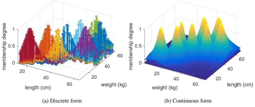
For example, based on the measured data, we can only derive the discrete εMFs from the three data clouds shown in Fig. 4. However, considering that weights and lengths are from a continuous domain based on common knowledge, the continuous εMFs can also be derived. The εFRB systems with discrete and continuous εMFs per feature are presented in Fig. 5(a) and (b) respectively.
(a) Discrete form (b) Continuous form
Fig.5. The examples of discrete and continuous εFRB system
(a) Discrete form (b) Continuous form
(c) Discrete “length” and continuous “weight” Fig.6. Visualization of 3D εMFs
Similar to the AnYa type FRB system, the proposed εFRB system is much more convenient and computationally simpler in high dimensional problems and it is unique in its ability to deal with problems containing categorical variables. This is thanks to the fact that only the prototypes are needed to be identified for the εFRB system (identified either by users or by the data-driven approach [11] ), and the system will derive εMFs from data clouds formed around the prototypes automatically.
higher (dozens, hundreds or more), A and T can also be larger. Therefore, the improvement is in orders of magnitude.
In the following two subsections, we will describe two approaches to identify the prototypes for the εFRB systems. The first one is using the newly introduced approach for forming data clouds [11], which is a nonparametric, entirely data-driven and objective method; the second one is based on human expertise.
3.2. Objective εFRB System Identification
In this subsection, we will describe the objective approach within the EDA framework for identifying the prototypes for the εFRB systems. The main procedure can be performed using the method for automatic formation of data clouds:
Step1: The multimodal densitiesDMM of all the data samples
K
x are calculated using equation (5).
For the specific example considered above, the multimodal densities DMM of the size of the 600 domestic dogs are depicted in Fig. 7 (a).
Step2: Find the unique data sample * 1
u with the maximum multimodal density DMM
u1* .Step 3: Remove u1* from
L
u and put it into
u *L, then set u1* as uR.Step 4: Find the nearest unique data sample * 2 u to R
u , remove * 2
u from
L
u and send * 2
u to
*L
u .
Step 5: Use u*2 as the new uR and repeat Step 4 until
Lu become empty.
Step 6: Rank the DMM of
*L
u according to their indexes from 1 to L. The ranked DMM are depicted in Fig. 7(b).
Step 7: Find the local maxima of the ranked
D
MM and use the corresponding unique data samples as prototypes,
p
. The local maxima of theD
MMare depicted in Fig.8.(a) Local maxima identified from the ranked DMM (b) Data samples with the local maximum DMM Fig.8. The local maxima of the ranked
D
MM for the illustrative exampleStep 8: Form data clouds from
K
x with
p using equation (11):
arg min ;
i i i K
cloud label
y p
x y x x (11)
Step 9: Obtain the centres
0
p from the data cloud.
Step 10: Calculate the multimodal densitiesDMM of
0
p using equation (5).
Step 11: Find out the centres satisfying the following condition and denote them as
1
p :
1
max | N ,
MM MM MM
i i i
i
IF D D D
THEN is a member of
p q q p p
p p
(12)
where
0
i
p p ;
Ni
p is the collection of data clouds whose centres are neighbouring topi:
N
j i j i
IF p p R THEN p p (13)
here
0
j
p p ;R 1
;
is the average Euclidean distance between any pair of centres;
is the corresponding standard deviation of the distances between the centres.Step 12: Set
1
p as
p .Step 14: Form data clouds from
K
x using
p . [image:15.595.253.488.111.323.2](a) The identified prototypes (red asterisks) (b) The data clouds formed around the prototypes Fig. 9. The final results
If now we consider the example used several times earlier, there are eight prototypes identified from the data and eight data clouds are formed around them. Based on the eight data clouds, eight εMFs are built, the εMFs are also depicted in Fig. 10 in a 3D form.
(a) Discrete form (b) Continuous form Fig. 10. Visualization of 3D continuous εMFs
[image:15.595.76.521.461.648.2]The common practice for the traditional machine learning approaches to process categorical variables is to map them to different integer numbers. For example, one may use digit “1” to represent job category “worker”, “2” to represent job category “teacher”, “3” to represent “policeman”, etc. Alternatively, one can use the 1-of-C encoding method [12] to map the categorical variables into a series of orthogonal binary variables like using “001” to represent job category “worker”, “010” to represent “teacher”, “100” to represent “policeman”, etc. However, no matter what kind of mapping is used, the encoding process always minimises the true differences between the data from different categories. This minimization is more obvious in high dimensional problems. In many cases, data from different categories are inconsistent and, in fact, incomparable. The best way for handling different categories is to process them separately and thus, avoid the interferences between each other.
Therefore, in the proposed approach, if the data contains A categories, the data is divided intoA groups based on their categories and used to form data clouds separately [11]. To be more specific, let us use the real climate dataset (temperature and wind speed) measured in Manchester, UK for the period 2010-2015 [13] for illustration. This dataset contains 479 samples obtained during the winter and 459 samples during the summer. As the dataset contains data samples from two categories (“winter” and “summer”), we firstly separate the two categories and then, form the data clouds using the technique described in [11] to find the prototypes from each category. As we can see from Fig.11, there are 21 prototypes identified from the 479 “winter” data samples and 24 prototypes identified from the 459 “summer” data samples.
(a) Winter (b) Summer
Fig.11. Prototypes identified from the data samples from the two categories (the black asterisks are the prototypes)
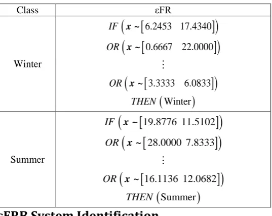
the εFRB system is identified based on the εFRs built upon the data clouds. The 3D visualization of the εMFs derived from data is depicted in Fig. 12. We also tabulate the εFRs in Table I for a better illustration.
[image:17.595.75.501.128.305.2] [image:17.595.164.433.365.578.2](a) Temperature (b) Wind speed Fig.12. 3D visualization of the εMFs
Table I. εFRs derived automatically from the real climate dataset
Class εFR
Winter
6.2453 17.4340
0.6667 22.0000
3.3333 6.0833
Winter
IF
OR
OR
THEN
x ~ x ~
x ~
Summer
19.8776 11.5102
28.0000 7.8333
16.1136 12.0682
Summer
IF
OR
OR
THEN
x ~ x ~
x ~
3.3. Subjective εFRB System Identification
(a) Three data clouds in 2D (b) 3D εMFs Fig.13. The εFRB system formed with the subjective approach
As it was mentioned in section 3.2 the real climate dataset contains two categories “winter” and “summer”. In order to build a highly descriptive εFRB system, for each category, one needs to select minimum one prototype in order to form at least one data cloud. For example, if we select two typical data samples prototype1=
8Co, 25mph
and prototype2= 2 Co,10mph measured in winter as the prototypes of the “winter” category,
and one typical data sample prototype3= 20 Co,11mph measured in summer as the prototype of the “summer” category. In this way, three data clouds are formed around the selected prototypes by the data samples associated with each one of these prototypes. They form Voronoi tessellation [11] and εFSs around these prototypes. The εFRB system with the three prototypes is visualized in a 3D form in Fig. 13.
As one can see, compared with defining the linguistic terms, prototypes, MFs, etc., one by one, the εFRB system only requires the prototypes to be defined, which is much simpler and easier. Instead of building mathematical models and handcrafting the whole FRB system piece by piece, the human experts/users only need to select few typical data samples as prototypes, and then the proposed method can autonomously build the εFRB system based on these prototypes. In this case, the prototypes have a clear meaning that: prototype1-cool and windy day;
prototype2-cold and quiet day; prototype3-warm and quiet day. The simplification in terms of human
involvement of the proposed approach can play a very important role in the collaboration between computer scientists and experts from different areas.
The convenience of the proposed approach may significantly influence the recommendation systems used by retailers. Let us use an example of buying a house. Of course, there are many visible and hidden factors to be considered before buying a new house, i.e. price, the distances to the city centre, schools and main roads, the environment, the safety conditions, the neighbourhood, house floor area, etc. To simplify this problem, we only consider four visible factors/features, i) price, ii) house floor area, iii) distance to the city centre and iv) distance to the schools.
Fig.14. The triangular type MFs of the traditional FRB system
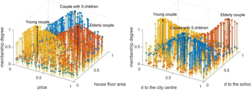
In contrast, when the εFRB system is used instead, the estate agent only needs to ask customers to select one or more houses they are most satisfied with. These houses can be any real houses in this city regardless whether they are for sale or not. These may also be imaginary, ideal houses as well. A family with five children may select one house that has large area and is very close to the schools, not far from the city centre and not expensive. A retired elderly couple may select a medium size house with luxury decoration and far away from the city centre and schools. A young couple may select a small economic house close to the city centre.
[image:20.595.78.507.291.448.2]Then, the selected houses can be used as prototypes to form the data clouds based on the four normalized variables from all the available for sale houses in the database. The εMFs derived from the data clouds formed around the prototypes are visualized in Fig. 15.
Fig. 15. Visualization of the εMFs based on four normalized attributes of houses (black asterisks represent the prototypes).
Based on the degrees of similarity of each available for sale house to the prototypes, the estate agent can easily make a list of recommended houses for each couple. All of this is achieved by asking the couples a simple question: “Can you, please, tell me the most satisfactory house in the city you have seen?” Similarly, each customer could also rank order few preferred houses, e.g. i) best; ii) good; iii) definitely no, etc.
4. Empirical Fuzzy Classifier
In this section, we will describe a new type of classifier based on the εFRs, named empirical fuzzy (εF) classifier and conduct numerical experiments to demonstrate the performance of the proposed classifier. The proposed εF classifier is very close to the concept of Naïve Bayes classifiers which perform classification based on the dominant per class likelihood expressed by a pre-defined (usually, Gaussian) pdf. It performs the classification based on the degree of membership of the εFRs (equation (9)) following the well-known “winner takes all” principle. However, other principles i.e. “few winners take all”, “fuzzily weighted”, “average” can also be considered depending on the specific problem.
As εFRs can be derived by both, the objective and subjective approaches, without losing generality, we use the objective approach as being described in section 3.2 for the εFRB system identification. Assuming that there have been N εFRs automatically derived from data using the technique for forming data clouds [11]. When applied to a new, unlabelled, unseen samplex, its label is given as:
1,2,..,
arg max MFi
i N
class label
x (14)
That is, the class label of x is decided by the label of the prototype that has higher membership degree.
To evaluate the performance of the proposed approach, three numerical examples based on benchmark datasets are conducted in this paper. The following algorithms were used in the comparison:
i) SVM classifier with Gaussian kernels [14], [15]; ii) SVM classifier with 4th Order Polynomial kernel [15]; iii) Naïve Bayes classifier [16];
iv) Decision tree classifier [17]; v) eClass0 classifier [18].
The comparison is based on the following criteria: i) Confusion matrix of the classification results;
ii) Average accuracy after 10 times Monte Carlo experiments;
iii) Average training time after 10 times Monte Carlo experiments (in seconds).
4.1. Wine Dataset
[19]
3) Ash; 4) Alkalinity of ash; 5) Magnesium; 6) Total phenols; 7) Flavonoids; 8) Neoflavanoid phenols; 9) Proanthocyanins; 10) Colour intensity; 11) Hue; 12) OD280/OD315of diluted wines; 13) Proline. Due to the high dimensionality, all the data samples are normalized by their norms in advance:
x
x
x (15)
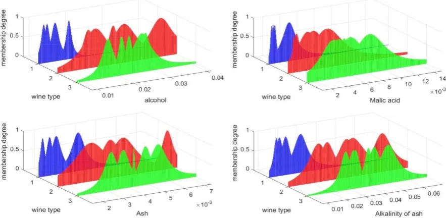
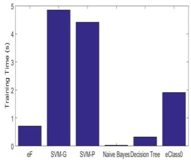
[image:22.595.70.528.271.406.2]We use the first 60% of the data samples of each class as the training set and use the rest of the dataset as the validation set. The classification results are tabulated in Table. II. For a better illustration, the εMFs of the first 4 attributes derived from the training samples are visualized in a 3D form per type per feature in Fig. 16.
Table. II Classification results on the wine dataset
Method True Class
Predicted
Accuracy Method True Class
Predicted
Accuracy
1 2 3 1 2 3
εFa
1 20 4 0
0.7324 Naïve Bayes
1 21 3 0
0.9437
2 1 22 5 2 0 27 1
3 3 6 10 3 0 0 19
SVM-Gb
1 0 24 0
0.3944 Decision tree
1 24 0 0
0.9718
2 0 28 0 2 2 26 0
3 0 19 0 3 0 0 19
SVM-Pc
1 18 6 0
0.6479 eClass0
1 21 1 2
0.6479
2 0 28 0 2 1 12 15
3 0 19 0 3 2 4 13
a
the proposed εF classifier b the SVM classifier with Gaussian kernel; c the SVM classifier with polynomial kernel
Fig. 16. The 3D visualization of the εMFs for the first 4 attributes of the wine dataset
[image:22.595.74.516.432.648.2]Fig.17. Overall accuracy Fig.18. Average training time (in seconds)
4.2. Banknote Authentication Dataset
[20]
Banknote authentication dataset was extracted from images that were taken from genuine and forged banknote-like specimens. Wavelet Transform tool was used to extract features from the images [21]. This dataset contains 1372 samples and each sample has four attributes:
1) variance of the wavelet transformed image; 2) skewness of the wavelet transformed image; 3) curtosis of the wavelet transformed image; 4) entropy of the image.
and one label: class (0 or 1). 762 of the data samples are in class 0 and 610 samples are in class 1.
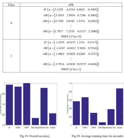
[image:23.595.302.496.77.236.2]We use the first 60% of the data samples of each class (152 samples from class 0 and 122 samples from class 1) as our training set and use the rest of the dataset as the validation set. The classification results obtained by the six classifiers are presented in Table III. The εFRs derived from the training data are presented as examples in Table IV for a better interpretability.
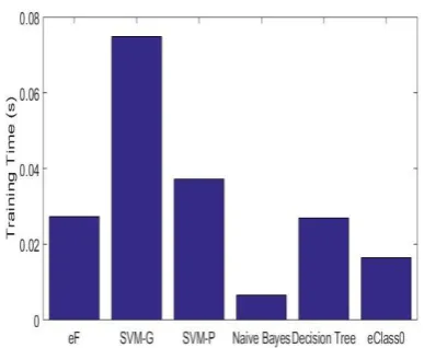
10 Monte Carlo experiments are also conducted on this dataset for further comparison. The average overall accuracies of the six classifiers are depicted in Fig. 19 and the corresponding average time consumption (in seconds) required for the training is presented in Fig. 20.
Table. III Classification results on the banknote authentication dataset
Method True Class
Predicted
Accuracy Method True Class
Predicted
Accuracy
0 1 0 1
εF 0 302 3 0.9945 Naïve
Bayes
0 278 21
0.8725
1 0 244 1 43 201
SVM-G 0 305 0 1.0000 Decision
tree
0 302 3
0.9891
1 0 244 1 2 241
[image:23.595.88.274.79.242.2]1 13 231 1 3 241
Table. IV The εFRs derived from the banknote authentication dataset
Class εFR
0
3.1229 -4.5316 4.4032 -0.1095 3.1019 2.9954 0.7296 0.3001 0.7350 5.8760 1.5374 -0.2825
1.7877 7.2335 -0.3137 -2.3080 0 IF OR OR OR THEN Class x ~ x ~ x ~ x ~ 1
-1.2555 -0.8157 1.1531 0.5117 -1.4167 -6.0412 5.5654 0.5516 -1.9863 -8.9029 8.8260 -0.3372
-3.7914 -6.9420 10.9737 -0.4656 1 IF OR OR OR THEN Class x ~ x ~ x ~ x ~
Fig.19. Overall accuracy Fig.20. Average training time (in seconds)
4.3. Tic-Tac-Toe Endgame Dataset
[22]
The Tic-Tac-Toe Endgame dataset contains a complete set of possible board configurations at the end of tic-tac-toe games. The target concept of this dataset is “winning for x”. This dataset contains 958 data samples with nine attributes and one class label [22]:
5) middle-middle-square: {x, o, b} 6) middle-right-square: {x, o, b} 7) bottom-left-square: {x, o, b} 8) bottom-middle-square: {x, o, b} 9) bottom-right-square: {x, o, b} 10) Class: {positive, negative}
In this experiment, we encode “x” as “1”, “o” as “5” and “b” as “3”. Obviously, all the variables are in the discrete domain. The data samples are normalized by their norms before classification using equation (15). The dataset is divided into two parts. We use the first 60% samples of each class for training, and the rest of them for validation. The classification results of the proposed classifier and the five comparative classifiers are tabulated in Table V.
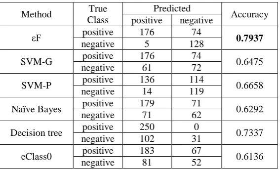
[image:25.595.157.441.438.610.2]We also conduct 10 Monte Carlo experiments by randomly selecting 60% of the data samples of each class for training the classifiers and using the rest for validating the classifiers. The average overall accuracy and the time consumption (in seconds) of the training process of the six classifiers are depicted in Fig. 21 and Fig. 22, respectively.
Table. V. Classification results on the Tic-Tac-Toe endgame dataset
Method True
Class
Predicted
Accuracy positive negative
εF positive 176 74 0.7937
negative 5 128
SVM-G positive 176 74 0.6475
negative 61 72
SVM-P positive 136 114 0.6658
negative 14 119
Naïve Bayes positive 179 71 0.6292
negative 71 62
Decision tree positive 250 0 0.7337
negative 102 31
eClass0 positive 183 67 0.6136
Fig.21. Overall accuracy Fig.22. Average training time (in seconds)
4.4. Letter Recognition Dataset
[23]
This dataset contains 20000 character images consisting of large numbers of black-and-white rectangular pixels displaying the 26 capital letters (from “A” to “Z”) of the Latin alphabet used in English language. Each image has been converted into 16 primitive numerical attributes as follows: 1) x-box: horizontal position of the box; 2) y-box: vertical position of the box; 3) width: width of the box; 4) height: height of the box; 5) onpix: total number of pixels that are “on”; 6) x-bar: mean value of x of the pixels that are “on” in the box; 7) y-bar: mean value of y of the pixels that are “on” in the box; 8) x2bar: mean value of the x variance; 9) y2bar:mean value of the y variance; 10) xybar: mean value of the x,y correlation; 11) x2ybr: mean value of the x·x·y; 12) xy2br: mean value of the x·y·y; 13) x-ege: mean edge count from left to right; 14) xegvy: correlation of x-ege with y; 15) y-ege: mean edge count from bottom to top; 16) yegvx: correlation of y-ege with x. The 16 attributes have been scaled to fit into a range of integer values from 0 through 15.
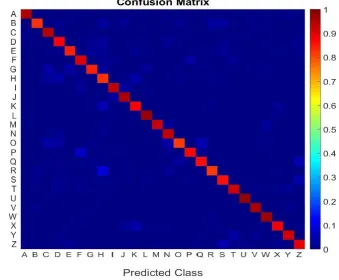
In this experiment, we, firstly, normalized the data samples by their norms before classification using equation (15). Then, the first 60% of the data samples of each class were used as a training set and the rest were used as a validation set. The confusion matrix of the result obtained by the proposed approach is depicted in Fig. 23. The εMFs of the 3rd and 4th attributes (width and height), derived from the training samples are visualized in a 3D
Fig. 23. The confusion matrix of the classification result of the letter recognition dataset
(b) εMF of the 4th attribute- height
Fig. 24. The 3D visualization of the εMFs of the letter recognition dataset
Same as the previous three benchmark problems, 10 Monte Carlo experiments are conducted by randomly selecting 60% of the data samples of each class for training the classifiers and using the rest for validating the classifiers. The average overall accuracy and the time consumption (in seconds) of the training process of the six classifiers are depicted in Fig. 25 and Fig. 26, respectively.
Fig.25. Overall accuracy Fig.26. Average training time (in seconds)
4.5. Discussion
5. Conclusion
In this paper, we introduce a new form of describing fuzzy sets, named εFSs and a new form of FRB systems, named εFRB grounded at the Empirical Data Analytics (EDA) framework. The proposed approach touches the fundamental question of how to build a FRB system. Two approaches (subjective and objective) for identifying εFRB systems are described in this paper. Through a number of illustrative examples, we demonstrate that the proposed approach is a powerful alternative for scientists working with FRB systems in various fields and it has a strong potential.
Compared with the traditional FSs and FRB systems, the proposed approach has the following significant advantages:
i) The εFSs are derived in a transparent, data-driven way without prior assumptions
ii) Effectively combines the data- and human- derived models; iii) It has very strong interpretability and high objectiveness;
iv) The involvement of human experts is significantly facilitated and can be bypassed.
Numerical examples in this paper have demonstrated the high performance of the εF classifier, but the applications of the proposed approach include, but are not limited to classification, control, prediction.
As a future work, we will detail the evolving εFRB systems, predictors and apply it to various problems, i.e. high frequency trading, image classification, aircraft control, etc. We will also prove stability conditions for the εFRB systems.
6. Acknowledgements
This work was partially supported by The Royal Society grant IE141329/2014 “Novel Machine Learning Paradigms to address Big Data Streams”.
Reference
[1] L. A. Zadeh, “Fuzzy sets,” Inf. Control, vol. 8, no. 3, pp. 338–353, 1965.
[2] P. Angelov, Autonomous Learning Systems: From Data Streams to Knowledge in Real Time. John Willey, 2012.
[3] E. H. Mamdani and S. Assilian, “An experiment in linguistic synthesis with a fuzzy logic controller,” Int. J. Man. Mach. Stud., vol. 7, no. 1, pp. 1–13, 1975.
[4] T. Takagi and M. Sugeno, “Fuzzy identification of systems and its applications to modeling and control,” IEEE Trans. Syst. Man. Cybern., vol. 15, no. 1, pp. 116–132, 1985.
[5] W. Pedrycz, “Fuzzy relational equations with generalized connectives and their applications,” Fuzzy Sets Syst., vol. 10, no. 1–3, pp. 185–201, 1983.
[6] P. Angelov and R. Yager, “A new type of simplified fuzzy rule-based system,” Int. J. Gen. Syst., vol. 41, no. 2, pp. 163–185, 2011.
10.1002/int.21899, 2017.
[9] C. C. Lee, “Fuzzy Logic in Control Systems : Fuzzy Logic Controller - Part 1,” IEEE Trans. Syst. Man Cybern., vol. 20, no. 2, pp. 404–418, 1990.
[10] A. Okabe, B. Boots, K. Sugihara, and S. N. Chiu, Spatial tessellations: concepts and applications of Voronoi diagrams, 2nd ed. Chichester, England: John Wiley & Sons., 1999.
[11] X. Gu, P. P. Angelov, and J. Principe, “Autonomous data partitioning,” under review, 2017.
[12] P. Cortez and A. Silva, “Using data mining to predict secondary school student performance,” in 5th Annual Future Business Technology Conference, 2008, pp. 5–12.
[13] “Climate Dataset in Manchester,” http://www.worldweatheronline.com.
[14] N. Cristianini and J. Shawe-Taylor, An Introduction to Support Vector Machines : and Other Kernel-Based Learning Methods. Cambridge: Cambridge University Press, 2000.
[15] J. H. Min and Y. C. Lee, “Bankruptcy prediction using support vector machine with optimal choice of kernel function parameters,” Expert Syst. Appl., vol. 28, no. 4, pp. 603–614, 2005.
[16] C. M. Bishop, Pattern Recognition. New York: Springer, 2006.
[17] S. R. Safavian and D. Landgrebe, “A survey of decsion tree clasifier methodology,” IEEE Trans. Syst. Man. Cybern., vol. 21, no. 3, pp. 660–674, 1990.
[18] P. Angelov and X. Zhou, “Evolving fuzzy-rule based classifiers from data streams,” IEEE Trans. Fuzzy Syst., vol. 16, no. 6, pp. 1462–1474, 2008.
[19] “Wine Dataset,” https://archive.ics.uci.edu/ml/datasets/Wine, Accessed on July 31st, 2017.
[20] “Banknote Authentication Dataset,” https://archive.ics.uci.edu/ml/datasets/banknote+authentication, Accessed on July 31st, 2017.
[21] V. Lohweg, J. L. Hoffmann, H. Dörksen, R. Hildebrand, E. Gillich, J. Hofmann, and J. Schaede, “Banknote authentication with mobile devices,” in Proc. SPIE 8665, Media Watermarking, Security, and Forensics 2013, 2013, pp. 866507–866507.
[22] “Tic-Tac-Toe Endgame Dataset,” https://archive.ics.uci.edu/ml/datasets/Tic-Tac-Toe+Endgame, Accessed on July 31st, 2017.