Some Studies on Convolution Neural Network

Some Studies on Convolution Neural Network

Goutam Sarker, PhD

Computer Science and Engineering Department, NIT Durgapur, INDIA

ABSTRACT

Two major tools to implement any artificial intelligence and machine learning systems are Symbolic AI and Artificial Neural Network AI. Artificial Neural Network (ANN) has made a tremendous improvement in the versatile area of Machine Learning (ML). Artificial Neural Network (ANN) is an assembly of huge number of weighted interconnected artificial neurons, initially invented with the inspiration of biological neurons. All these models are much better than previous models implemented with symbolic AI so far as their performance is concerned. One revolutionary change in ANN is Convolutional Neural Network (CNN). These structures are mainly suitable for complex pattern recognition tasks within images for the purpose of computer vision.

General Terms

Artificial Intelligence, Artificial Neural Network, Machine Learning, Pattern Recognition

Keywords

Convolution Neural Network, Deep Learning, Optical Character Recognition, Machine Transcription, Machine Translation, Accuracy

1.

INTRODUCTION

To extract different patterns within various images for the specific task of image recognition, the latest state of the art technique is to design and develop a Convolutional Neural Network (CNN) [1,2,3]. In this method, the specific features of images are suitably extracted and coded in that special type of neural network, with the learned or programmed filters or kernels. These filters or kernels are specific to particular images. This makes the CNN [4,5,6,14] a far better concept and methodology for complex pattern and image recognition tasks, providing so far the best effectiveness and efficiency.

In our previous works for Face Detection and Localization [15,16,17,21,26] we used probabilistic framework and supervised learning method to perform Face Detection and Localization. In [18,27] an unsupervised learning model for both Face Identification and Localization is implemented. A modified RBF Network with basis function learning by Optimal Clustering is for Face Identification and Localization is utilized in [19,20,28,29,30,31]. A Modified RBFN with basis function learning with a new concept of Heuristic Based Clustering is used in [22,24,25] while a Competitive Learning Network using Malsburg Learning is employed for Face Detection and Localization in [23].

In all those previous works we used classical ANN to solve in general any pattern recognition problem like Face Detection, Identification and Localization and person authentication with biometrics. But conventional ANN has some limitations also.

Classical ANN is having the severe limitations in that, the time complexity of computation for the purpose of pattern recognition in image processing is too large to afford.

Let us take one example of learning and recognizing image MNIST benchmark handwritten dataset. Each digit of the dataset is having the dimensionality of 28*28. If we employ a conventional classical neural network, any neuron of the first hidden layer should have 28*28*1= 784 weighted links falling onto it. Here we have considered conversion of MNIST data set to just black and white. This ‘784’ number is moderate and affordable. This is just because of the fact, that this does not demand the network size to be extremely large enough to accommodate it.

But if our input image is a coloured one of size 128*128, any neuron in the first hidden layer should have 128*128*3 = 12288 weighted links landing onto it. (Multiplication of pixel size by 1 for black and white image while multiplication by 3 for coloured image). This number is much larger than the previous black and white one. Therefore all the neurons in the first hidden layer would have 12288 weighted links. Accordingly the size of the classical neural network for the purpose of recognition of coloured normalized MINST digit demands to be abnormally large enough. Apparently to cope with this situation, we may think to increase the size of the network (by just increasing the number of hidden layers and the number of neurons per hidden layer). But there are two major problems in doing so. They are mentioned as follows:

1.) The first problem is that, if the network size is extremely large, it accordingly demands enormously huge computational power as well as the learning and recognition time to make the system learn and recognize the input data set.

2.) The second problem is the problem of overfitting. The power of generalisation is severely reduced with overfitting. The overfitting occurs if the network size is large. If the network size is large, the memorization power of the network undesirably increases, thereby dropping down the capability of generalization. Also extremely large number of weights are to be learned by the network – because the storage capacity of the network is large. Network power of generalization reduces and thereby the network will overfit. This degrades the performance of the system so far as the image recognition is capabilities are concerned. Thus increasing the network size cannot be a solution for handling large coloured image.

2.

THE FUNDAMENTALS OF

CONVOLUTION

Consider the above system is a very noisy one. We want to obtain a more accurate noise free position of the same aircraft. Then we have to make an average of several such measurements of position p(t). The more the measurement is recent, the more it is likely to be close to an accurate one. With that there must be an weight attached to each measurement – the weights are assigned to more recent measurements.

So let us present a new function P that will give an accurate estimate of the position of the aircraft where

P(t) =

∫

p(t) w(t) dt

This technique to find the most accurate position of the aircraft is in general the basic concept of the operation of convolution.

We can also denote the operation of convolution through another similar symbolic notation

P(t) = (p*w)(t)

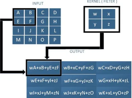
With respect to convolutional neural network, the first argument i.e. the function ‘p’ is referred to as the input, while the second argument i.e. the weight function ‘w’ is called the kernel or filter. The output is called feature map or activation map. The ‘w’ should definitely be a valid probability density function otherwise we will not be able to perform the operation of convolution.

Fig. 1 A 2D convolution without kernel flipping – the sliding kernel always lies entirely within the image,

making the convolution a valid one

Fig. 1 shows a 2D convolution without kernel flipping. Here the kernel or the filter moves left to right and top to bottom, by one pixel and each time produces the dot product of the local region of the input and the kernel. The moving or sliding kernel always lies within the image boundary.

Kernel Non Flipping – The kernel while sliding on the input always lies entirely within the input region boundary.

Kernel Flipping – The kernel while sliding on the input moves beyond the input region boundary.

3.

MOTIVATIONS FOR

CONVOLUTIONAL NEURAL

NETWORK (CNN)

The architecture of Convolutional Neural Network (CNN) [6,7,8] in general is comprised of a series of the set of some convolutional layers, rectified linear unit layer, pooling layer. In convolutional layer, to perform the operation of

convolution, some filters or kernels are employed

Fig. 2 In case of CNN, the input output connections are always sparse.

.Classical or conventional ANNs are much improved and empowered with the three major concepts or ideas of Convolution Neural Network. These are the main features of any CNN [9,10]. These are as mentioned below:

1. Sparse Connectivity.

2. Sharing of Parameters.

3. Equivariant Representation.

3.1

Sparse

Connectivity

(or

Sparse

Interactions or Sparse Weights)

Fig. 3. An example of sparse input output connection

Fig. 4 Variation of output for the same input in case of a sparse connectivity and a full connectivity

In Fig. 4 One input X3 is active and by this all the output units in S that are affected by this active input unit are highlighted. The upper diagram is showing the output S formed by convolution of kernel width 3, where only 3 output units are affected by X3, since the connections are sparse. The lower diagram is showing the output S formed by matrix multiplication, where all the inputs are connected to all the output neurons. Thus all the output neurons are affected by input neuron X3.

3.2

Sharing of Parameters or Weights:

In classical or conventional neural network, to compute the output of any layer, each weight of the weight matrix is used only once. This weight is multiplied by the corresponding input vector component and becomes totally useless for the

Network, each component of the kernel as well as the entire kernel itself is moved along the input activation and thereby used at each and every position of the input (Some extreme boundary pixels of the input might be discarded according to some design considerations). In some design consideration the kernel might move a few pixels of the input beyond the boundary producing a ‘kernel flipping’. On the contrary in other design the kernel movement is restricted only within the input region producing ‘kernel non flipping’. The sharing of parameters or weights has the advantage that rather than learning a separate parameter or weight set for different locations of the input, the system learns only one set in the form of kernel or filter.

3.3

Equi Variant Representation:

The overall output corresponding to an input is same, if the sequence of operation applied to the input is interchanged – this property is termed as Equi Variance.

Mathematically, a function ‘f’ is equi variant to a function ‘g’, if f(g(x) ) = g(f(x)). For convolution operation, if ‘f’ is a function that convolves the input and ‘g’ is another function that translates the input (i.e. shifts the input from one position to another), then convolution function ‘f’ is equi variant to ‘g’.

4.

BROAD ARCHITECTURE OF CNN

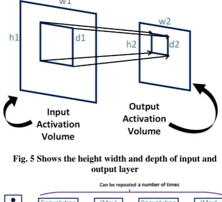
In general in CNN there are three different types of layers namely – convolution layer, pooling layer and fully connected layer. The convolution layer is comprised of input volume, kernel or filter and output volume. The input and output volume with height, width and depth is indicated in Fig. 5. The convolution and pooling layers may be repeated a number of times to get the desired size of activation map. When these are combined together, a complete CNN structure is formed. The complete overall architecture of CNN is indicated in Fig. 6.

Fig. 5 Shows the height width and depth of input and output layer

Fig. 6. The overall architecture of CNN

1. Convolution Layer: Local regions of the input volume are connected to the output neurons for the purpose of convolution. Convolution layer computes the output of the neurons connected to the local regions of the input volume. This is mathematically done by scalar product of the weights of the kernel and the local region connected to the input volume.

2. Rectified Linear Unit (ReLU): The ReLU applies an activation function (e.g. sigmoid or g(z) = max{0,z}) to each an every element at the output volume produced by the previous layer.

3. Pooling Layer: Sub sampling along the spatial dimensionality of the given input (produced as an activation map at the output volume or as an output of ReLU) further reduces the number of parameters within the activation map. This sub sampling is called pooling.

In general, max pooling with a pooling kernel dimensionality of 2*2 is applied to the activation map produced by Convolution Layer. The number of pixels, through which the pooling kernel has to be shifted along the spatial dimensionality (formally called kernel stride) is usually set as 2 for a kernel dimensionality of 2*2, so that there is no overlappling. With this evidently the activation map produced by the convolution layer is scaled down to 25% (because 2*2 = 4 pixels are represented by 1 pixel at the output).

One variation of pooling is Overlapped Pooling. This occurs when the kernel size is more than the stride. For example, say the stride is set as 2 and the kernel size is 3*3. In this case the pooling would be overlapped.

Pooling definitely distorts the image and therefore a pooling kernel size above 3*3 distorts heavily the input image and thereby degrades the desirable performance of the CNN.

The advantage of pooling is to reduce the size of the image and number of parameters. Also the pooling makes the representation more or less invariant to small translation of the overall input image. We will see it later in section 5.

4. Fully Connected Layer: Here neurons are connected between two adjacent layers, without being connected to any neuron in any layer within them – unlike Recurrent Neural Network (RNN)

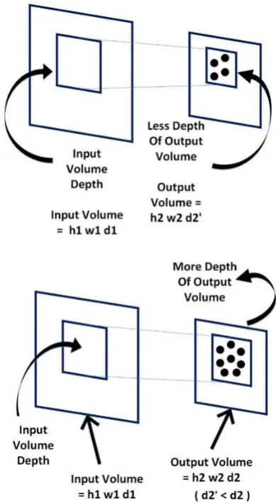
Hyper Parameters : Depth, Stride and Zero Padding: We can optimize the Convolutional Layer Output with three hyper parameters namely depth, stride and zero padding. They are detailed as below:

1) Depth : The number of neurons within a layer of the output volume connected to the same region of the input is called the depth of the output volume produced during convolution. The lesser is the value of this hyper parameter the lesser is the number of neurons and parameters in the network. But lowering the value of this hyperparameter also degrades the overall performance of the CNN so far as the pattern recognition capability is concerned. The hyper parameter depth is indicated in both upper and lower parts of Fig. 7, where for the same input volume depth, the upper part is has less depth while the lower part has more depth in output volume.

Fig. 7 Depth of the input and output volume

2) Stride: This is the number of pixels through which the kernel (filter) has to be shifted around the spatial dimensionality of the input. If the stride is set as 1, then a heavily overlapped receptive field is obtained and extremely large activations and large output spatial dimensions are yielded.

On the contrary, if the stride is set to be a number greater than 1, then the amount of overlapping is comparatively smaller than before and an output of lower activations and lower spatial dimensions are produced.

we need zero padding. With this the outer region of the input volume is surrounded by few layers of zero.

Fig. 8 Input vector, Pooled Vector Kernel and Destination Pixel

Fig. 8 shows one specimen input vector, pooled vector and kernel or filter. A local region of size 3*3 of input is highlighted and produces a pooled vector. The kernel produces a dot product and creates an activation in the destination pixel. The kernel with a stride lands on next local region and produces another pooled vector. Similarly the activation of next destination pixel is created.

In the case the stride = 1, if the input volume size is m*n, the kernel size is r*r, then the output volume size is [m-(r-1)]. Thus for example, if we want to keep output volume size = input volume size = m*n, in case the kernel size is r*r, then we are to put (r-1) layers of zero padding surrounding the input (of course the stride should be equal to one). Similarly we can also make the output volume size larger than the input volume size, by suitably increasing the amount of zero padding. Thus by controlling the amount of zero padding, we can make the output volume size (height and width) either greater than or equal to or less than the input volume size.

To extract the different desirable features of the input image, a number of learned or programmed filters or kernels are employed. A corresponding activation map is generated by each kernel. Those activation maps are accumulated or stacked together. This produces the complete set of output volume of the convolution layer.

For example, if there are n kernels or filters then there are n activation map which produces the complete output volume. If it is a coloured image, then there are n*3 kernels or filters, thereby 3 channels per activation map; and thus n*3 activation maps.

5.

ADVANTAGES OF POOLING

Pooling introduces:

1. Translation Invariance.

2. Rotation Invariance.

3. Scaling Invariance.

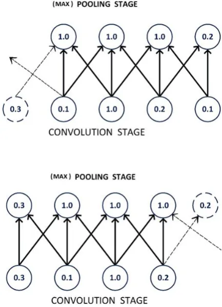
Translation Invariance: If the input image is slightly translated to a new position, then also it is perfectly detected due to pooling stage of CNN. Below is a simple example:

Fig. 9 Max pooling introduces translation invariance

In the upper part of fig. 9, the bottom row is the output of nonlinear convolution stage. The result of (max) pooling is indicated by upper row. Here we have considered a stride of unity. Since the pooling kernel size is 3 and stride is 1 (which is less than 3), this is an example of over lapped pooling.

In the lower part of the fig. 9, the input has been translated towards right by one pixel. The corresponding values of all the pixels of the bottom row are changed due to this shifting. But in the figure just half of the values of the activations of the top row have changed. This is due to the reason that max pooling units accumulate the maximum value in a neighbourhood, irrespective of the exact location of the maximum value.

Rotation Invariance: If the input image is slightly rotated by some angle, then also it is perfectly detected due to pooling stage of CNN. Fig. 10 is a simple example:

Fig. 10 Rotation invariance through max pooling

vertically upward and the third one is rotated clockwise by and angle of 45 deg. These all kernels are supposed to detect a handwritten “B”. When a 45 deg anticlockwise rotated “B” is placed as input image, large activation is produced in the activation map corresponding to Filter 1. Similarly when a 45 deg clockwise rotated “B” is placed as input image, large activation is produced in the activation map corresponding to Filter 3. In the first part of the figure, the pooling of the activation corresponding to Filter 1 would be maximum, while that of the other two would be minimum. In the second part of the figure, the pooling of the activation corresponding to Filter 3 would be maximum, while that of the other two would be minimum. But when these three pooled activations are integrated together, the integrator would indicate large activation irrespective of which pooled activation created large response. Thus the integrator of the pooled outputs would have large activation, irrespective of any of the above orientation of “B” given as input. Thereby all those differently oriented “B”s are successfully detected as “B” only.

Scaling Invariance: Through convolution with or without suitable zero padding and pooling, the input image is suitably scaled up or down as desired.

In conclusion, the major advantage of convolution is to overcome the effect of rotation, translation and scaling during for the purpose of efficient, effective and successful image recognition.

6.

AN EXAMPLE OF CONVOLUTION

AND MAX POOLING

In Fig. 11 we are going to present one 6*6 image input and two kernels or filters, namely Filter 1 and Filter 2, which are expected to grab or extract two different features likely to be present in various locations of the given input image.

Here Filter 1 represents one particular feature, while Filter 2 represents another particular feature, which are expected to be present in different locations of the input image. The size of the pattern or feature detected by both of them is equal to 3*3.

Fig. 11 One sample 6*6 Input Image

Filter 1 produces an activation map or feature map in the output volume as shown in Fig. 12:

Fig. 12 First feature map corresponding to first filter

Fig. 13 Second feature map corresponding to second filter

In case the stride is equal to one, the size of the activation or feature map in the output volume = {m-(r-1)} = {6-(3-1)} = 4*4; because the input image size is m*m = 6*6, kernel size is r*r = 3*3. Note that there is no zero padding in the input.

If there is a zero padding of z layers in the original input, then, the size of the activation or feature map in the output volume = {(m+z) – (r-1)}. As for example, if the zero padding z =1, and kernel size = 3*3, for the same input image of size = 6*6, then the activation map size in the output volume = {(6+1) – (3-1)} = 5*5. Here we have assumed that the stride is equal to one as before.

Output volume is a stack of different activation maps produced by different kernels. One activation map or feature map describes the different locations in the input where a particular feature represented by a filter of kernel is present. When we repeat the process for each filter, we get a series of activation map to produce the complete output volume.

7.

COLOUR IMAGE

In all previous examples we considered monochrome image. There a particular feature in the input image is described by one and only one filter. Thus one filter is sufficient to extract that feature.

Fig. 14 Colour image feature/ activation map corresponding to two filters

8.

MAX POOLING

The idea of max pooling is to extract the maximum activation out of the pooling region, indicated by the pooling kernel.

There are other varieties of pooling apart from Max Pooling. Another common pooling is known as L2 pooling. Here we don’t take the maximum activation of say 2*2 region. Unlike this we take the square root of the sum of squares of the activations within the 2*2 region. Both Max Pooling and L2 pooling are widely used. Sometimes other types of pooling such as average pooling may be used

Let us consider that we are using the two filters of Fig. 15 as indicated below :

Fig. 15 Two filters used for creation of two activation maps

Corresponding feature maps or activation maps in the output volume for the two filters are shown below in Fig. 16.

Fig. 16 Two feature maps corresponding to two filters given as input to Max Pooling unit

Now suppose we perform a max pooling with a pooling kernel size = 2*2. The stride of the pooling kernel is equal to two (and not one), so that this is no overlapping during the pooling process. The max pooling output is indicated in the below mentioned Fig. 17.

Fig. 17 Max pooling output corresponding to two feature maps

Pooling is also sometimes called sub sampling. Pooling usually compresses the original image or make the original image size smaller. But it cannot change one image to another.

In the above example two 4*4 image (actually activation or feature map which is input to the pooling stage) is compressed into two 2*2 image due to the effect of pooling. So the compression ratio of pooling is = 4*4 / 2*2 = 2

In general if the activation map size is m*n and the pooling kernel size is p*q, assuming there is no overlapping during pooling, the compression ratio is given by the following formula:

C = m*n / p*q

number and number of parameter needed at subsequent layers are thereby substantially reduced. Fig. 18 indicates a particular input is convolved with two filters and max pooled producing two activation maps.

Fig. 18 Each filter is a channel and creates a separate activation (feature) map and a new smaller image through pooling

9.

MAX POOLING

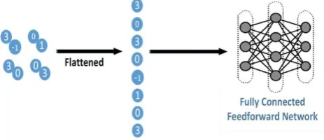
Convolution and max pooling may be repeated a number of times to get the desired size of the reduced image. This has to be flattened and finally applied as input to the fully connected network to detect the output class. This is shown below in Fig. 19.

Fig. 19 A series of convolution and max pooling

Final pooling output is a stack of activations corresponding to different filters. These when serialized or flattened would be a one dimensional matrix. This is the input to the fully connected network as shown below in Fig. 20

Fig. 20 An example of max pooling and corresponding flattening

Fig. 21 Convolution Neural Network (CNN) instructions for Convolution and Pooling in Keras

Fig. 22 Convolution Neural Network (CNN) Architecture in Keras

The network has input image of size 28*28 neurons. These are the pixel intensities for the MNIST data set image. Then a convolution layer with 25 kernels each of size 3*3 (this is also the size of the local receptive field) follows this. This results 25*26*26 hidden feature neurons. The next step is to perform max pooling with a max pooling kernel size 2*2 with a stride of 2 (no overlapping) across all the 25 feature or activation maps. The result is a layer of 25*13*13 hidden feature neurons. The process of convolution and max pooling is once again repeated, but this time with 50 kernels of size as before i.e. 3*3. With this, convolution layer yields a layer of 50*11*11 hidden feature neurons, while the max pooling layer yields a layer of 50*5*5 hidden feature neurons. This is now flattened at the next layer.

The prime advantage of Sharing of Weights is that it heavily reduces the number of parameters involved in a convolution neural network. If the kernel size is 3*3 as before, for each feature map we need 9 = 3*3 shared weights. If there are 25 feature maps, during first convolution we need 25*3*3 = 225 parameters. Similarly during second convolution we need 50*3*3 = 450 parameters, since during that convolution we had 50 feature maps. Thus altogether we need 675 parameters. These many parameters are needed up to the first hidden layer neuron of fully connected network. On the contrary if we use only a fully connected network without convolution, with 28*28=784 input neurons, and assuming a modest 30 hidden layer neurons, we require 784*30 = 23520 parameters even for only the first hidden layer neuron. Thus, approximately 35 times more number of parameters are needed in fully connected layer, in comparison to that of convolutional layer.

10.

CONCLUSION

The present paper is an introduction to Convolutional Neural Network (CNN)- one revolutionary and dramatic concept in Artificial Neural Network (ANN). Starting with the preliminary concepts and motivations of CNN, the paper broadly discusses the general architecture of any CNN, the different layers and components of CNN, the major advantages of CNN over classical ANN. It also details some specific CNN architectures. The author expects that the beginners of CNN will find this paper a most helpful one.

11.

ACKNOWLEDGEMENTS

The author would like to thank his M.Tech Project Student Ms. Swagata Ghosh, Computer Science and Engineering Department, NIT Durgapur for drawing all the figures in the paper.

12.

REFERENCES

[1] Ian Goodfellow and Yoshua Bengio and Aaron Courville: Deep Learning, MIT Press.

[2] Ciresan, D.C., Meier, U., Gambardella, L.M., Schmidhuber, H.: Convolutional neural network committees for handwritten character classification. In:Document Analysis and Recognition (ICDAR), 2011 International Conference on. Pp 1135-1139, IEEE(2011).

[3] Farabet, C., Martini, B., Akselrod, P., Talay, S., LeCun, Y., Culurciello, E.: Hardware accelerated convolutional neural networks for synthetic vision systems. In:Circuits and Systems (ISCAS). Proceedings of 2010 IEEE International Symposium on. Pp 257-260. IEEE (2010)

[4] Karpathy, A. Toderici, G., Shetty, S., Leung, T., Sukthankar, R., Fei-Fei, L.: Large scale video classification with convolutional neural networks. In: Computer Vision and Pattern Recognition (CVPR), 2014 IEEE Conference on. Pp. 17ng,

[5] T., Sukthankar, R., Fei-Fei, L.: Large scale video classification with convolutional neural networks. In: Computer Vision and Pattern Recognition (CVPR), 2014 IEEE Conference on. Pp. 1725-1732. IEEE(2014).

[6] Nebaaer, C.: Evaluation of convolutional neural networks for visual recognition. Neural Networks, IEEE Transactions on 9(4), 685-696 (1998).

[7] Simard, P.Y., Steinkraus, D., Platt, J,C.: Best practices for convolutional neural networks applied to visual document analysis. In: null. P. 958. IEEE(2003).

[8] Szarvas, M., Yoshizawa, A., Yamamoto,M., Ogata, J.:Pedestrain detection with convolutional neural networks. In: Intelligent Vehicles Symposium, 2005. Proceedings. IEEE. Pp. 224-229. IEEE(2005).

[9] Szegedy, C., Toshev, A., Erhan, D. : Deep neural networks for object detection. In: Advances in Neural Information Processing Systems. Pp. 2553-2561 (2013).

[10] Tivive, F.H.C., Bouzerdoum, A. : A new class of convolutional neural networks (siconnets) and their applications of face detection. In: Neural Networks, 2003. Proceedings of the International Joint Conference on. Vol. 3, pp 2157-2162. IEEE(2003).

[11] Zeiler, M.D., Fergus, R.:Stochastic pooling for regularization of deep convolutional neural networks. arXiv preprint arXiv: 1301.3557(2013).

[12] Zeiler, M.D., Fergus, R.: Visualizing and understanding convolutional networks. In: Computer Vision – ECCV 2014, pp. 818-833. Springer (2014)

[13] Sarker, G.(2000),A Learning Expert System for Image Recognition, Journal of The Institution of Engineers (I), Computer Engineering Division.,Vol. 81, 6-15.

[14] Mehak and Tarun Gulati, Detection of Digital Forgery Image using Different Techniques, International Journal of Engineering Trends and Technology (IJETT) – Volume 46 Number 8 April 2017.

[15] G. Sarker(2010),A Probabilistic Framework of Face Detection , International Journal of Computer,

Information Technology and Engineering

(IJCITAE),4(1), 19-25.

[16] G. Sarker(2011),A Multilayer Network for Face Detection and Localization, International Journal of Computer, Information Technology and Engineering (IJCITAE), 5(2), 35-39.

[17] G. Sarker(2012),A Back Propagation Network for Face Identification and Localization, International Journal of Computer, Information Technology and Engineering (IJCITAE),6(1), 1-7.

[18] G. Sarker(2012), An Unsupervised Learning Network for Face Identification and Localization, International Journal of Computer, Information Technology and Engineering (IJCITAE),6(2), 83-89.

[19] G. Sarker and K. Roy (2013), A Modified RBF Network With Optimal Clustering For Face Identification and Localization, International Journal of Advanced Computational Engineering and Networking, ISSN: 2320-2106.,1(3), 30 -35.

[20] G. Sarker and K. Roy(2013), An RBF Network with Optimal Clustering for Face Identification, Engineering Science International Research Journal (ISSN) – 2300 – 4338 ,1(1),ISBB: 978-93-81583-90-6, 70-74.

[21] G. Sarker(2013), An Optimal Back Propagation Network for Face Identification and Localization, International Journal of Computers and Applications (IJCA),ACTA

Press, Canada.,35(2).,DOI 10.2316 / Journal

.202.2013.2.202 – 3388.

Computer Information Technology and Engineering (IJCITAE), Serials Publications ,8(2),109-118.

[23]G. Sarker(2014), A Competitive Learning Network for Face Detection and Localization, International Journal of Computer Information Technology and Engineering (IJCITAE), Serials Publications, 8(2),119-123.

[24] G. Sarker(2002), A Semantic Concept Model Approach for Pattern Classification and recognition, 28th Annual

Convention and Exhibition IEEE – ACE

2002.,December 20-21 2002 , Science City ,Kolkata, 271 – 274.

[25]G. Sarker(2005), A Heuristic Based Hybrid Clustering for Natural Classification in Data Mining, 20th Indian Engineering Congress, organized by The Institution of Engineers (India), December 15-18, 2005, Kolkata, INDIA, paper no. 4.

[26]G. Sarker(2011), A Back propagation Network for Face Identification and Localization, 2011 International Conference on Recent Trends in Information Systems (ReTIS–2011) held in Dec. 21-23, Kolkata, DOI: 10.1109/ReTIS.2011.6146834, pp 24-29.

[27] G. Sarker(2012), An Unsupervised Learning Network for Face Identification and Localization, 2012 International Conference on Communications, Devices and Intelligent Systems (CODIS) Dec. 28 and

29, 2012, Kolkata, DOI:

10.1109/CODIS.2012.6422282, pp 652- 655.

[28] G. Sarker, and K. Roy(2013), An RBF Network with Optimal Clustering for Face Identification, International Conference on Information & Engineering Science – 2013(ICIES -2013), Feb. 21-23 2013, organized by IMRF, Vijayawada, Andhra Pradesh, pp – 70-74.

[29] G. Sarker and K. Roy(2013), A Modified RBF Network with Optimal Clustering for Face Identification and Localization, International Conference on Information & Engineering Science – 2013(ICIES -2013), Feb. 21-23 2013, organized by IMRF, Vijayawada, Andhra Pradesh

pp 32-37.

[30] K. Roy and G. Sarker (2013), A Location Invariant Face Identification and Localization with Modified RBF Network, International Conference on Computer and Systems ICCS-2013, 21-22 September, 2013, pp – 23-28, Bardhaman.