Computationally Efficient Problem Reformulations for Capacitated Lot Sizing Problem

(1)

ISSN Online: 2160-8849 ISSN Print: 2160-8830

DOI: 10.4236/ajor.2018.84018 Jul. 18, 2018 312 American Journal of Operations Research

Computationally Efficient Problem

Reformulations for Capacitated

Lot Sizing Problem

Renduchintala Raghavendra Kumar Sharma, Priyank Sinha, Mananjay Kumar Verma

Industrial and Management Engineering Department, IIT Kanpur, Kanpur, India

Abstract

In this article, we propose novel reformulations for capacitated lot sizing problem. These reformulations are the result of reducing the number of va-riables (by eliminating the backorder variable) or increasing the number of constraints (time capacity constraints) in the standard problem formulation. These reformulations are expected to reduce the computational time com-plexity of the problem. Their computational efficiency is evaluated later in this article through numerical analysis on randomly generated problems.

Keywords

Capacitated Lot Sizing Problem, Efficient Problem Formulation, Branch and Bound

1. Introduction

Lot sizing problem aims to optimally utilize the available production resources while meeting the demand targets. It is classified as medium-term planning in production planning taxonomy. Lot sizing problem formulation depends upon the layout and the operating constraints in the production system. In the manu-facturing industry, we come across many types of production systems. These production systems further give rise to different types of lot sizing problems (with different constraints and operating conditions) and their solution metho-dologies. Hence there is a rich literature on lot sizing problem and their solution methods. In this article, we restrict our discussion to general dynamic mul-ti-level capacitated lot sizing problem.

This problem was first proposed by Billington et al.[1]. It addresses the fol-lowing scenario: a finite planning horizon is given and is divided into discrete

How to cite this paper: Sharma, R.R.K., Sinha, P. and Verma, M.K. (2018) Compu-tationally Efficient Problem Reformulations for Capacitated Lot Sizing Problem. Amer-ican Journal of Operations Research, 8, 312-322.

https://doi.org/10.4236/ajor.2018.84018

Received: June 11, 2018 Accepted: July 15, 2018 Published: July 18, 2018

http://creativecommons.org/licenses/by/4.0/

(2)

DOI: 10.4236/ajor.2018.84018 313 American Journal of Operations Research

time periods. There is a dynamic demand for items which needs to be satisfied for each time period while honoring the production capacity constraints. Prob-lem aims to develop a production plan over all time periods while minimizing the total cost comprising of setup cost, inventory cost, and backordering cost.

A capacitated lot sizing problem is a well-known NP-hard problem. If the ca-pacity constraints of the problem are relaxed, then the problem can be solved in polynomial time [2]. Many model formulations have been proposed to develop an efficient numerical solution. These formulations differ with each other due to variables and constraints used. Formulations given in this article belongs to in-ventory and lot-size (I & L) formulations category, which are among the most popular in the literature due to their computational efficiency. These formula-tions use production quantity and inventory levels as the variables. Relaxation of each constraint in the standard I&L model affects the problem structure and hence its numerical complexity. Relaxation of capacity constraints decomposes CLSP into single-level lot sizing problem popularly known as Wagner-Whitin problem [2]. Further, some popular extensions to the standard problem have been suggested in the literature, to address certain practical issues. For example, Dillenberger et al.[3] have extended the problem to incorporate setup carryover. A setup cost and setup time are not incurred if the same item is being produced in the next time period, carried forward by the previous period. Our formulation incorporates binary variable for setup to address these issues. Binary setup vari-able to address the carryover of setup to the next period was earlier used by Hasse [4], and Surie and Stadtler [5].

We next discuss certain problem reformulations from the literature which are computationally efficient. CLSP can be formulated to assign each production quantity to a demand in a specific time period while minimizing the production cost. Shortest route formulation was proposed by Eppen and Martin [6] for a single level case. It was later extended by Tempelemier and Helber [7] for mul-ti-level CLSP. Stadtler proposed an improvement in this formulation ([8] [9]), which decreases the number of non-negative coefficients. Rosling [10] intro-duced a formulation based on Plant location problem analogy. This formulation was further extended by Maes et al.[11] for the capacitated case of a lot-sizing problem. Capacity constraints were included in the original formulation for this purpose. Equivalence of Shortest route and SPL formulation in terms of objec-tive function was shown by Denizel et al. [12].

(3)

valid inequalities for multi-level capacitated lot sizing problem with set up carry over. Setup carryover constraints are redefined to achieve a computational ad-vantage in this formulation.

Research in this article is based on the appropriate reformulation of the stan-dard capacitated lot sizing problem. We state the stanstan-dard problem formulation and then derive three reformulations of the problem by eliminating the backor-dering variable or/and adding two capacity constraints. Efficacies of these for-mulations in terms of reduced computational complexity are demonstrated through numerical analysis of random problems on GAMS.

2. Research Methodology

As stated in the previous section, we intend to evaluate the improvement in computational efficiency of the model when the number of decision variables are decreased, or constraints are added to tighten the bound of the solution space. Model A1 is the reference standard model, which is tinkered to develop model A2, A3, and A4 accordingly. In model A2 (proposed later), we have eliminated the backordering variable; hence it is expected to be computationally efficient when compared with model A1. Similarly, we have added two extra constraints (Equation (27), Equation (28)) in our standard model (A1) which is referred to as model A3. Further, we eliminate backordering variable while adding two con-straints in model A1 and refer it to model A4. Hence model A4 is expected to perform best among all. Efficacy of each model is evaluated by performing paired t-test of the computational time of random problem instances on A1, A2, A3, and A4. Branch and bound method is used in GAMS for solving random problem optimally by these models. Finally it is concluded in section 6 that most computationally efficient formulation should be used solving capacitated lot sizing problem.

3. Problem Formulation/Reformulation

Table 1. Notations used in the model.

Indices used T Set of time periods.

t Particular time period such that t T∈ . I Set of products to be produced. i Particular product such that i I∈ .

Constants

it

CP Unit cost of producing i in the period t.

it

CS Unit cost of setup for the item i in the period t.

it

CINV _{Unit cost of holding inventory of item i for period 1.}

it

CBO _{Unit cost of backordering item i demanded during the period t.}

it

(4)

DOI: 10.4236/ajor.2018.84018 315 American Journal of Operations Research Continued

t

CAPT_{Capacity available in time units in the period t.}

it

D Demand for the item i during the period t.

it

PT Time required for processing the item i.

i

ST Time required for setting up the production for the item i.

Definition of Variables

it

XP Number of items i to be produced in the period t.

it

XINV _{Number of items i carried as inventory to be produced during the period t.}

it

XBO _{Number of item i that will be backordered from the period t.}

it

YS Binary setup variable.

3.1. Model A1

[

]

1 1

Minimize I T it* it it* it it* it it* it i t

Z CP XP CS YS CINV XINV CBO XBO

= =

=

∑∑

+ + + ₍₁₎

Subject to:

, 1 , 1 ,

it i t it it it i t

XP XINV+ − +XBO =D +XINV +XBO − ∀ ∈i I t T∈ (2)

(

)

1 * *

I

it it i it t

i= PT XP ST YS CAPT t T

+ ≤ ∀ ∈

∑

₍₃₎

(

)

1 * *

I

it it i it t

i= PT D ST YS CAPT t T

+ ≤ ∀ ∈

∑

₍₄₎

,

it it it

XP CAP YS≤ ∀ ∈i I t T∈ ₍₅₎

1 1

T T

it it

t= XP t= D i I

≥ ∀ ∈

∑

(6)

0 0

i

XINV = ∀ ∈i I₍₇₎

0

iT

XINV = ∀ ∈i I₍₈₎

0 0

i

XBO = ∀ ∈i I₍₉₎

0

iT

XBO = ∀ ∈i I₍₁₀₎

{ }

0,1 ,

it

YS ∈ ∀ ∈i I t T∈ ₍₁₁₎

, , 0 ,

it it it

XINV XP XBO ≥ ∀ ∈i I t T∈ ₍₁₂₎

3.2. Model A2

[

]

1 1

1

1 1

1 1 1 1

Minimize * * *

* I T

it it it it it it

i t

t t

T I

it it it it

t i t t

Z CP XP CS YS CINV XINV

CBO D XINV XP

= = = = = = = + +   + _ + − _  

∑∑

∑

(13)

Subject to:

1 1

1 1 0 ,

t t

it it it

t= D XINV t= XP i I t T

+ − ≥ ∀ ∈ ∈

(5)

(

)

1 * *

I

it it i it t

+ ≤ ∀ ∈

∑

(15)

,

it it it

XP CAP YS≤ ∀ ∈i I t T∈ ₍₁₆₎

1 1

T T

it it

t= XP t= D i I

≥ ∀ ∈

∑

(17)

0 0

i

XINV = ∀ ∈i I₍₁₈₎

0

iT

XINV = ∀ ∈i I ₍₁₉₎

{ }

0,1 ,

it

YS ∈ ∀ ∈i I t T∈ ₍₂₀₎

, 0 ,

it it

XINV XP ≥ ∀ ∈i I t T∈ ₍₂₁₎

3.3. Model A3

[

]

1 1

Minimize I T it* it it* it it* it it* it i t

Z CP XP CS YS CINV XINV CBO XBO

= =

=

∑∑

+ + + ₍₂₂₎

Subject to:

, 1 , 1 ,

it i t it it it i t

XP XINV+ − +XBO =D +XINV +XBO − ∀ ∈i I t T∈ (23)

(

)

1 * *

I

it it i it t

+ ≤ ∀ ∈

∑

(24)

(

)

1 * *

I

it it i it t

i= PT D ST YS CAPT t T

+ ≤ ∀ ∈

∑

(25)

,

it it it

XP CAP YS≤ ∀ ∈i I t T∈ ₍₂₆₎

(

)

1 1 * * 1

I T T

it it i it t

i= t= PT D ST YS t= CAPT

+ ≤

∑∑

∑

(27)

(

)

1 1 * * 1

I T T

it it i it t

i= t= PT XP ST YS t= CAPT

+ ≤

∑∑

∑

(28)

1 1

T T

it it

t= XP t= D i I

≥ ∀ ∈

∑

(29)

0 0

i

XINV = ∀ ∈i I₍₃₀₎

0

iT

XINV = ∀ ∈i I ₍₃₁₎

0 0

i

XBO = ∀ ∈i I₍₃₂₎

0

iT

XBO = ∀ ∈i I ₍₃₃₎

{ }

0,1 ,

it

YS ∈ ∀ ∈i I t T∈ ₍₃₄₎

, , 0 ,

it it it

XINV XP XBO ≥ ∀ ∈i I t T∈ ₍₃₅₎

3.4. Model A4

[

]

1 1

1

1 1

1 1 1 1

Minimize * * *

* I T

it it it it it it

i t

t t

T I

it it it it

t i t t

Z CP XP CS YS CINV XINV

CBO D XINV XP

= = = = = = = + +   + _ + − _  

∑∑

(6)

Subject to:

1 1

1 1 0 ,

t t

it it it

t= D XINV t= XP i I t T

+ − ≥ ∀ ∈ ∈

∑

(37)

(

)

1 * *

I

it it i it t

+ ≤ ∀ ∈

∑

(38)

,

it it it

XP CAP YS≤ ∀ ∈i I t T∈ ₍₃₉₎

(

)

1 1 * * 1

I T T

it it i it t

i= t= PT D ST YS t= CAPT

+ ≤

∑∑

∑

(40)

(

)

1 1 * * 1

I T T

it it i it t

i= t= PT XP ST YS t= CAPT

+ ≤

∑∑

∑

(41)

1 1

T T

it it

t= XP t= D i I

≥ ∀ ∈

∑

(42)

0 0

i

XINV = ∀ ∈i I₍₄₃₎

0

iT

XINV = ∀ ∈i I ₍₄₄₎

{ }

0,1 ,

it

YS ∈ ∀ ∈i I t T∈ ₍₄₅₎

, 0 ,

it it

XINV XP ≥ ∀ ∈i I t T∈ ₍₄₆₎

Problem notations are tabulated in Table 1. Equation (1), Equation (13), Eq-uation (22), and EqEq-uation (36) minimize the total production cost of the system in model A1, A2, A3, and A4 respectively. Equation (2), Equation (14), Equation (23), and Equation (37) are the state equations as they ensure that the total quantities in a particular time period is a function of total quantities carried forward from the preceding time period while satisfying demand. It must be noted that in model A2 and A4, the backorder variable has been eliminated from the model by appropriate substitution (backorder variable XBOit, has been

(7)

only for individual time period. Equation (6), Equation (17), Equation (29), and Equation (42) ensures that demand is satisfied in each period. Equations (7)-(10), Equation (18), Equation (19), Equations (30)-(33), Equation (43), Equation (44) sets the initial and final conditions (boundary conditions) over the production horizon. Equation (11), Equation (12), Equation (20), Equation (21), Equation (34), Equation (35), Equation (45), Equation (46) are the binary and non-nega- tivity constraints for decision variables.

4. Numerical Experiments

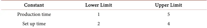
[image:7.595.209.540.325.447.2]

40 problems each of size 5 × 5 and 6 × 6 are randomly generated in GAMS. 5 × 5, 6 × 6 problems denotes the lot sizing problem to find an optimum production plan of 5 items over 5 time periods, and 6 items over 6 time periods respectively. Only feasible problems are retained for data analysis (6 × 6—29 problems, 5 × 5—31 problems). Value of constants in these problems is randomly generated according to normal distribution (Table 2) and uniform distribution (Table 3).

Table 2. Random data generation (Normal distribution).

Constant Mean Standard Deviation Unit cost of set up 100 2 Unit cost of Back Order 100 2 Unit Cost of Production 200 2 Unit Cost of Holding Inventory 200 2 Capacity (Production resource) 30 2

Demand 10 2

Capacity (time) 400 2

Table 3. Random data generation (Uniform Distribution).

Constant Lower Limit Upper Limit

Production time 1 5

Set up time 2 4

5. Data Analysis

All the problems are implemented in GAMS. Solution to these sample problems are tabulated in Appendix. According to t-test performed on data, problem A3 is computationally efficient to problem A1 with a statistical significance of 0.009317 (p-value). Similarly A4 is better than A2 with a statistical significance of 0.003071 (p-value). Model A2 is computationally more efficient than model A1 with a statistical significance of 0.000695 (p-value). Model A4 is computa-tionally more efficient than model A3 with a statistical significance of 0.00473 (p-value).

6. Conclusion

[image:7.595.208.539.479.524.2]

(8)

va-DOI: 10.4236/ajor.2018.84018 319 American Journal of Operations Research

riables, increasing the number of constraints on the computational time of lot sizing problem through 4 models. We infer from our data analysis that model A4 is the most computationally efficient model, and hence is recommended to be used for solving capacitated lot sizing problem.

References

[1] Billington, P.J., McClain, J.O. and Joseph Thomas, L. (1983) Mathematical Pro-gramming Approaches to Capacity-Constrained MRP Systems: Review, Formula-tion and Problem ReducFormula-tion. Management Science, 29, 1126-1141.

https://doi.org/10.1287/mnsc.29.10.1126

[2] Wagner, H.M. and Whitin, T.M. (1958) Dynamic Version of the Economic Lot Size Model. Management Science, 5, 89-96. https://doi.org/10.1287/mnsc.5.1.89

[3] Dillenberger, C., Escudero, L.F., Wollensak, A. and Zhang, W. (1993) On Solving a Large-Scale Resource Allocation Problem in Production Planning. Operations Re-search in Production Planning and Control, Springer, Berlin, 105-119.

https://doi.org/10.1007/978-3-642-78063-9_7

[4] Haase, K. (2012) Lotsizing and Scheduling for Production Planning. Vol. 408, Sprin-ger Science & Business Media.

https://books.google.co.in/books?hl=en&lr=&id=QVL-CAAAQBAJ&oi=fnd&pg=P A1&dq=Lotsizing+and+scheduling+for+production+planning&ots=HSTSWCFLR T&sig=nDlJCwQpjGkD0DPWZUGI2RMa3Kg#v=onepage&q=Lotsizing%20and%2 0scheduling%20for%20production%20planning&f=false

[5] Suerie, C. and Stadtler, H. (2003) The Capacitated Lot-Sizing Problem with Linked Lot Sizes. Management Science, 49, 1039-1054.

https://doi.org/10.1287/mnsc.49.8.1039.16406

[6] Eppen, G.D. and Kipp Martin, R. (1987) Solving Multi-Item Capacitated Lot-Sizing Problems Using Variable Redefinition. Operations Research, 35, 832-848.

https://doi.org/10.1287/opre.35.6.832

[7] Tempelmeier, H. and Helber, S. (1994) A Heuristic for Dynamic Multi-Item Mul-ti-Level Capacitated Lotsizing for General Product Structures. European Journal of Operational Research, 75, 296-311. https://doi.org/10.1016/0377-2217(94)90076-0

[8] Stadtler, H. (1996) Mixed Integer Programming Model Formulations for Dynamic Multi-Item Multi-Level Capacitated Lotsizing. European Journal of Operational Research, 94, 561-581. https://doi.org/10.1016/0377-2217(95)00094-1

[9] Stadtler, H. (1997) Reformulations of the Shortest Route Model for Dynamic Mul-ti-Item Multi-Level Capacitated Lotsizing. Operations-Research-Spektrum, 19, 87-96.

https://doi.org/10.1007/BF01545506

[10] Rosling, K. (1986) Optimal Lot-Sizing for Dynamic Assembly Systems. Multi-Stage Production Planning and Inventory Control, Springer, Berlin, 119-131.

https://doi.org/10.1007/978-3-642-51693-1_7

[11] Maes, J., McClain, J.O. and Van Wassenhove, L.N. (1991) Multilevel Capacitated Lotsizing Complexity and LP-Based Heuristics. European Journal of Operational Research, 53, 131-148. https://doi.org/10.1016/0377-2217(91)90130-N

[12] Denizel, M., Tevhide Altekin, F., Süral, H. and Stadtler, H. (2008) Equivalence of the LP Relaxations of Two Strong Formulations for the Capacitated Lot-Sizing Problem with Setup Times. OR Spectrum, 30, 773-785.

https://doi.org/10.1007/s00291-007-0094-3

(9)

Mul-DOI: 10.4236/ajor.2018.84018 320 American Journal of Operations Research ti-Item Capacitated Lot Sizing. Management Science, 30, 1255-1261.

[14] Pochet, Y. and Wolsey, L.A. (1991) Solving Multi-Item Lot-Sizing Problems Using Strong Cutting Planes. Management Science, 37, 53-67.

[15] Clark, P.W. and Armentano, L.E. (1997) Replacement of Alfalfa Neutral Detergent Fiber with a Combination of Nonforage Fiber Sources. Journal of Dairy Science, 80, 675-680. https://doi.org/10.3168/jds.S0022-0302(97)75986-1

(10)

Appendix: Data Analysis Results

(a)

(11)

(b)