Flexible Text Segmentation with Structured Multilabel Classification
Ryan McDonald Koby Crammer Fernando Pereira
Department of Computer and Information Science University of Pennsylvania
Philadelphia, PA 19104
{ryantm,crammer,pereira}@cis.upenn.edu
Abstract
Many language processing tasks can be re-duced to breaking the text into segments with prescribed properties. Such tasks include sentence splitting, tokenization, named-entity extraction, and chunking. We present a new model of text segmenta-tion based on ideas from multilabel clas-sification. Using this model, we can natu-rally represent segmentation problems in-volving overlapping and non-contiguous segments. We evaluate the model on en-tity extraction and noun-phrase chunking and show that it is more accurate for over-lapping and non-contiguous segments, but it still performs well on simpler data sets for which sequential tagging has been the best method.
1 Introduction
Text segmentation is a basic task in language pro-cessing, with applications such as tokenization, sen-tence splitting, named-entity extraction, and chunk-ing. Many parsers, translation systems, and extrac-tion systems rely on such segmentaextrac-tions to accu-rately process the data. Depending on the applica-tion, segments may be tokens, phrases, or sentences. However, in this paper we primarily focus on seg-menting sentences into tokens.
The most common approach to text segmenta-tion is to use finite-state sequence tagging mod-els, in which each atomic text element (character
or token) is labeled with a tag representing its role in a segmentation. Models of that form include hidden Markov models (Rabiner, 1989; Bikel et al., 1999) as well as discriminative tagging mod-els based on maximum entropy classification (Rat-naparkhi, 1996; McCallum et al., 2000), conditional random fields (Lafferty et al., 2001; Sha and Pereira, 2003), and large-margin techniques (Kudo and Mat-sumoto, 2001; Taskar et al., 2003). Tagging mod-els are the best previous methods for text segmen-tation. However, their purely sequential form limits their ability to naturally handle overlapping or non-contiguous segments.
We present here an alternative view of segmenta-tion as structured multilabel classificasegmenta-tion. In this view, a segmentation of a text is a set of segments, each of which is defined by the set of text positions that belong to the segment. Thus, a particular seg-ment may not be a set of consecutive positions in the text, and segments may overlap. Given a text
x = x1· · ·xn, the set of possible segments, which
corresponds to the set of possible classification la-bels, is seg(x) = {O,I}n; fory ∈seg(x),yi =I iff xi belongs to the segment. Then, our segmen-tation task is to determine which labels are correct segments in a given text. We have thus a structured multilabel classification problem: each instance, a text, may have multiple structured labels, represent-ing each of its segments. These labels are structured in that they do not come from a predefined set, but instead are built from sets of choices associated to the elements of arbitrarily long instances.
More generally, we may be interested in typed segments, e.g. segments naming different types of
entities. In that case, the set of segment labels is seg(x) = T × {O,I}n, where T is the set of
seg-ment types. Since the extension is straightforward, we frame the discussion in terms of untyped seg-ments, and only discuss segment types as needed.
At first sight, it might appear that we have made the segmentation problem intractably harder by turn-ing it into a classification problem with a number of labels exponential on the length of the instance. However, we can bound the number of labels under consideration and take advantage of the structure of labels to find thekmost likely labels efficiently. This will allow us to exploit recent advances in online dis-criminative methods for multilabel classification and ranking (Crammer and Singer, 2002).
Though multilabel classification has been well studied (Schapire and Singer, 1999; Elisseeff and Weston, 2001), as far as we are aware, this is the first study involving structured labels.
2 Segmentation as Tagging
The standard approach to text segmentation is to use tagging techniques with a BIO tag set. Elements in the input text are tagged with one of Bfor the be-ginning of a contiguous segment, I for the inside of a contiguous segment, or O for outside a seg-ment. Thus, segments must be contiguous and non-overlapping. For instance, consider the sentence Es-timated volume was a light 2.4 million ounces. Fig-ure 1a shows how this sentence would be labeled using the BIO tag set for the problem of identifying base NPs in text. Given a particular tagging for a sentence, it is trivial to find all the segments, those whose tag sequences are longest matches for the reg-ular expression BI∗. For typed segments, the BIO tag set is easily augmented to indicate not only seg-ment boundaries, but also the type of each segseg-ment. Figure 1b exemplifies the tags for the task of finding people and organizations in text.
Sequential tagging with the BIO tag set has proven quite accurate for shallow parsing and named entity extraction tasks (Kudo and Matsumoto, 2001; Sha and Pereira, 2003; Tjong Kim Sang and De Meulder, 2003). However, this approach can only identify non-overlapping, contiguous seg-ments. This is sufficient for some applications, and in any case, most training data sets are annotated
without concern for overlapping or non-contiguous segments. However, there are instances in which se-quential labeling techniques using the BIO label set will encounter problems.
Figure 2 shows two simple examples of segmen-tations involving overlapping, non-contiguous seg-ments. In both cases, it is difficult to see how a sequential tagger could extract the segments cor-rectly. It would be possible to grow the tag set to represent a bounded number of overlapping, non-contiguous segments by representing all possible combinations of segment membership overk over-lapping segments, but this would require an arbitrary upper bound onkand would lead to models that gen-eralize poorly and are expensive to train.
Dickinson and Meurers (2005) point out that, as language processing begins to tackle problems in free-word order languages and discourse analysis, annotating and extracting non-contiguous segmen-tations of text will become increasingly important. Though we focus primarily on entity extraction and NP chunking in this paper, there is no reason why ideas presented here could not be extended to man-aging other non-contiguous phenomena.
3 Structured Multilabel Classification
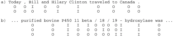
As outlined in Section 1, we represent segmentation as multilabel classification, assigning to each text the set of segments it contains. Figure 3 shows the segments for the examples of Figure 2. Each seg-ment is given by aO/Iassignment to its words, in-dicating which words belong to the segment.
By representing the segmentation problems as multilabel classification, we have fundamentally changed the objective of our learning and inference algorithms. The sequential tagging formulation is aimed to learn and find the best possible tagging of a text. In multilabel classification, we train model parameters so that correct labels — that is, correct segments – receive higher score than all incorrect ones. Likewise, inference becomes the problem of finding the set of correct labels for a text, that is, the set of correct segments.
Sec-a. Estimated volume was a light 2.4 million ounces .
B I O B I I I I O
b. Bill Clinton and Microsoft founder Bill Gates met today for 20 minutes .
B-PER I-PER O B-ORG O B-PER I-PER O O O O O O
Figure 1: Sequential labeling formulation of text segmentation using the BIO label set. a) NP-chunking tasks. b) Named-entity extraction task.
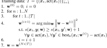
a) Today, Bill and Hilary Clinton traveled to Canada. - Person: Bill Clinton
- Person: Hilary Clinton
b) ... purified bovine P450 11 beta / 18 / 19 - hydroxylase was ... - Enzyme: P450 11 beta-hydroxylase
[image:3.612.311.533.270.369.2]- Enzyme: P450 18-hydroxylase - Enzyme: P450 19-hydroxilase
Figure 2: Examples of overlapping and non-contiguous text segmentations.
tion 3.2, we describe a polynomial-time inference algorithm for finding up tokcorrect segments.
3.1 Training Multilabel Classifiers
Our model is based on a linear scores(x,y;w) for
each segmentyof textx, defined as
s(x,y;w) =w·f(x,y)
where f(x,y) is a feature vector representation of
the sentence-segment pair, and w is a vector of feature weights. For a given text x, act(x) ⊆
seg(x)denotes the set of correct segments forx, and
bestk(x;w)denotes the set ofksegments with
high-est score relative to the weight vector w. For learn-ing, we use a training setT ={(xt,act(xt))}|T |t=1 of
texts labeled with the correct segmentation.
We will discuss later the design of f(x,y)and an
efficient algorithm for finding thekhighest scoring segments (where k is sufficiently large to include all correct segments). In this section, we present a method for learning a weight vector w that seeks to score correct segments above all incorrect segments. Crammer and Singer (2002), extended by Cram-mer (2005), provide online learning algorithms for multilabel classification and ranking that take one instance at a time, construct a set of scoring con-straints for the instance, and adjust the weight vec-tor to satisfy the constraints. The constraints en-force a margin between the scores of correct labels and those of incorrect labels. The benefits of large-margin learning are best known from SVMs (Cris-tianini and Shawe-Taylor, 2000; Sch¨olkopf and
Training data:T ={(xt,act(xt))}|T |t=1 1. w(0)= 0; i= 0
2. forn: 1..N 3. fort: 1..|T |
4. w(i+1)= arg minw ‚ ‚
‚w−w
(i)‚‚ ‚
2
s.t.s(xt,y;w)≥s(xt,y0;w) + 1
∀y∈act(xt),∀y0∈bestk(xt;w(i))−act(xt)
6. i=i+ 1
7. w=w(N∗|T |)
Figure 4: A simplified version of the multilabel learning algorithm of Crammer and Singer (2002).
Smola, 2002), and are analyzed in detail by Cram-mer (2005) for online multilabel classification.
al-a) Today , Bill and Hilary Clinton traveled to Canada .
O O I O O I O O O O
O O O O I I O O O O
b) ... purified bovine P450 11 beta / 18 / 19 - hydroxylase was ...
O O I I I O O O O I I O
O O I O O O I O O I I O
[image:4.612.70.440.54.136.2]O O I O O O O O I I I O
Figure 3: Correct segments for two examples.
gorithm (Censor and Zenios, 1997).
Using standard arguments for linear classifiers (add constant feature, rescale weights) and the fact that all the correct scores in line 4 of Figure 4 are re-quired to be above all the incorrect scores in the top k, that line can be replaced by
w(i+1)= arg minw
w−w(i) 2
s.t.s(xt,y;w)≥1ands(xt,y0;w)≤ −1
∀y∈act(xt),∀y0 ∈bestk(xt;w(i))−act(xt)
If v is the number of correct segments for x,
this transformation replacesO(kv)constraints with O(k+v)constraints: segment scores are compared to a single positive or negative threshold rather then to each other. At test time, we find the segments with positive score by finding thekhighest scoring segments and discarding those with a negative score.
3.2 Inference
During learning and at test time we require a method for finding thek highest scoring segments. At test time, we predict as correct all the segments with pos-itive score in the top k. In this section we give an algorithm that calculates this precisely.
For inference, tagging models typically use the Viterbi algorithm (Rabiner, 1989). The algorithm is given by the following standard recurrences:
S[i, t] = maxt0s(t0, t, i) +S[i−1, t0]
B[i, t] = arg maxt0s(t0, t, i) +S[i−1, t0]
with appropriate initial conditions, where s(t0, t, i)
is the score for going from tag t0 at i−1 to tag t ati. The dynamic programming tableS[i, t]stores the score of the best tag sequence ending at posi-tioniwith tag t, andB[i, t] is a back-pointer to the previous tag in the best sequence ending at iwith t, which allows us to reconstruct the best sequence. The Viterbi algorithm has easyk-best extensions.
We could find thekhighest scoring segments us-ing Viterbi. However, for the case of non-contiguous segments, we would like to represent higher-order dependencies that are difficult to model in Viterbi. In particular, in Figure 3b we definitely want a feature bridging the gap between Bill and Clinton, which could not be captured with a standard first-order model. But moving to higher-order models would require adding dimensions to the dynamic program-ming tablesSandB, with corresponding multipliers to the complexity of inference.
To represent dependencies between non-contiguous text positions, for any given segment
y = y1· · ·yn, let i(y) = 0i1· · ·im(n+ 1)be the increasing sequence of indicesij such thatyij =I, padded for convenience with the dummy first index
0 and last index n+ 1. Also for convenience, set x0 = -s- and xn+1 = -e- for fixed start and
end markers. Then, we restrict ourselves to feature functions f(x,y)that factor relative to the input as
f(x,y) =
|i(y)| X
j=1
g(i(y)j−1, i(y)j) (1)
wherei(y)j is thejthinteger ini(y)and g is a
fea-ture function depending on arbitrary properties of the input relative to the indicesi(y)j−1andi(y)j.
Applying (1) to the segment Bill Clinton in Fig-ure 3, its score would be
w·[g(0,3) +g(3,6) +g(6,11)]
This feature representation allows us to include de-pendencies between non-contiguous segment posi-tions, as well as dependencies on any properties of the input, including properties of skipped positions.
We now define the following dynamic program
These recurrences compute the scoreS[i]of the best partial segment ending at ias the sum of the max-imum score of a partial segment ending at position j < i, and the score of skipping from j toi. The back-pointer tableBallows us to reconstruct the se-quence of positions included in the segment.
Clearly, this program requires O(n2) time for a text of lengthn. Furthermore we can easily augment this algorithm in the standard fashion to find the k best segments, and multiple segment types, result-ing in a runtime ofO(n2kT), whereTis the number of types. O(n2kT)is not ideal, but is still practical since in this work we are segmenting sentences. If we can bound the largest gap in any non-contiguous segment by a constantg n, then the runtime can be improved to O(ngkT). This runtime does not compare favorably to the standard Viterbi algorithm that runs in O(nT2), especially for largek. How-ever, we found that for even large k we could still train large models in a matter of hours and test on unseen data in a few minutes.
3.2.1 Restrictions
Often a segmentation task or data set will restrict particular kinds of segments. For instance, it may be the case that a data set does not have any overlap-ping or non-contiguous segments. Embedded seg-mentations – those in which one segment’s tokens are a subset of another’s – is also a phenomenon that sometimes does not occur.
It is easy to restrict the inference algorithm to dis-allow such segments if they are unnecessary. For ex-ample, if two segments overlap or are embedded, the inference algorithm can just return the highest scor-ing one. Or it can simply ignore all non-contiguous segments if it is known that they do not occur in the data. In Section 4 we will augment the inference algorithm accordingly for each data set.
3.3 Feature Representation
We now discuss the design of the feature function for two consecutive segment positions g(j, i), where j < i. We build individual binary-valued features from predicates over the input, for instance, the iden-tities of words in the sentence at particular posi-tions relative toiand j. The selection of predicates varies by task, and we provide specific predicate sets in Section 4 for various data sets. In this section,
we use for illustration word-pair identity predicates such asxj =Bill&xi=Clinton.
For sequential tagging models, predicates are combined with the set of states (or tags) to create a feature representation. For our model, we define the following possible states:
start ≡ j= 0
end ≡ i=n+ 1
next ≡ j=i−1
skip ≡ j < i−1
For example, the following features would be on for g(0,3)1and g(3,6), respectively, in Figure 3a:
xj =-s-&xi =Bill&start xj =Bill&xi=Clinton&skip
These features indicate a predicate’s role in the seg-ment: at the beginning, at the end, over contiguous segment words or skipping over some words. All features can be augmented to indicate specific seg-ment types for multi-type segseg-mentation tasks. No matter what the task, we always add predicates that represent ranges of the distancei−j, as well as what words or part-of-speech tags occur between the two words. For instance, g(3,6)might contain
word-in-between=and&skip
These features are designed to identify common characteristics of non-contiguous segments such as the presence of conjunctions or punctuation in skipped portions. Although we have considered only binary features here, the model in principle allows arbitrary real-valued feature.
3.4 Summary
We presented a method for text segmentation that equates the problem to structured multilabel classi-fication where each label corresponds to a segment. We showed that learning and inference can be man-aged tractably in the formulation by efficiently find-ing the k highest scoring segments through a dy-namic programming algorithm that factors the struc-ture of each segment. The only concern is that k must be large enough to include all correct segments,
1Note that “skip” is not on for g(0,3)even thoughj < i−1.
which we will discuss further in Section 4. This method naturally models all possible segmentations including those with overlapping or non-contiguous segments. Out approach can be seen as multilabel variant of the work of McDonald et al. (2004), which creates a set of constraints to separate the score of the single correct output from thek highest scoring outputs with an appropriate large margin.
4 Experiments
We now describe a set of experiments on named en-tity and base NP segmentation. For these experi-ments, we set k = n, wheren is the length of the sentence. This represents a reasonable upper bound on the number of entities or chunks in a sentence and results in a time complexity ofO(n3T).
We compare our methods with both the averaged perceptron (Collins, 2002) and conditional random fields (Lafferty et al., 2001) using identical predicate sets. Though all systems use identical predicates, the actual features of the systems are different due to the fundamental differences between the multilabel classification and sequential tagging models.
4.1 Standard data sets
Our first experiments are standard named entity and base NP data sets with no overlapping, embedded or non-contiguous segments. These experiments will show that, for simple segmentations, our model is competitive with sequential tagging models.
For the named entity experiments we used the CoNLL 2003 (Tjong Kim Sang and De Meulder, 2003) data with people, organizations, locations and miscellaneous entities. We used standard predicates based on word, POS and orthographic information over a previous to next word window. For the NP chunking experiments we used the standard CoNLL 2000 data set (Kudo and Matsumoto, 2001; Sha and Pereira, 2003) using the predicate set defined by Sha and Pereira (2003).
The first three rows of Table 1 compare the mul-tilabel classification approach to standard sequen-tial classifiers. As one might expect, the perfor-mance of the multilabel classification method is be-low that of the sequential tagging methods. This is because those methods model contiguous segments well without the need for thresholds ork-best
infer-ence. In addition, the multilabel method shows sig-nificantly higher precision then recall. One possible reason for this is that during the course of learning, the model will see many segments that are nearly correct, e.g., segments that overlap correct segments and differ by a single token. As a result, the model learns to score all segments containing even a small amount of negative evidence as invalid in order to ensure that these nearly correct segments have a suf-ficiently low score.
One way to alleviate this problem is to restrict the inference algorithm to not return any overlapping, non-contiguous or embedded segmentations as dis-cussed in Section 3.2.1, since this data set does not contain segments of this kind. This way, the learning stage only updates the parameters when a nearly cor-rect segment actually out scores the corcor-rect one. The results of this system are shown in row 4 of Table 1. We can see that this change did lead to a more bal-anced precision/recall, however it is clear that more investigation is required.
4.2 Chemical substance extraction
The second set of experiments involves extract-ing chemical substance names from MEDLINE ab-stracts that relevant to the inhibition of the enzyme CYP450 (PennBioIE, 2005). We focus on abstracts that have at least one overlapping or non-contiguous annotation. This data set contains 6164 annotated chemical substances, including 6% that are both overlapping and non-contiguous. Figure 3b is an example from the corpus. We use identical predi-cates to the named entity experiments in Section 4.1. Though the data does contain overlapping and non-contiguous segments, it does not contain embedded segments. Results are shown in Table 2 using 10-fold cross validation. The sequential tagging models were trained using only sentences with no overlap-ping or non-contiguous entities. We found this pro-vided the best performance. Row 4 of Table 2 shows the multilabel approach with the inference algorithm restricted to not allow embedded segments.
a. Named-Entity Extraction b. NP-chunking
Precision Recall F-measure Precision Recall F-measure
Avg. Perceptron 82.46 83.14 82.80 94.22 93.88 94.05
CRFs 83.36 83.57 83.47 94.57 94.00 94.29
Multilabel 92.47 74.19 82.33 94.65 92.28 93.45
Multilabel with Restrictions 91.08 76.68 83.26 94.10 93.70 93.90
Table 1: Results for named-entity extraction and NP-chunking on data sets with only non-overlapping and contiguous segments annotated.
Chem Substance Extraction - A Chem Substance Extraction - B
Precision Recall F-measure Precision Recall F-measure
Avg. Perceptron 82.98 79.40 81.15 1.0 0.0 0.0
CRFs 85.85 79.06 82.31 1.0 0.0 0.0
Multilabel 88.24 80.84 84.38 62.56 33.67 43.78
[image:7.612.161.504.53.120.2]Multilabel with Restrictions 88.55 84.59 86.53 72.58 45.92 56.25
Table 2: Results for chemical substance extraction. Table A is for all entities in the data set and Table B is only for those entities that are overlapping and non-contiguous.
4.3 Tuning Precision and Recall
The learning algorithm in Section 3.1 seeks a sep-arator through the origin, though, our experimental results suggest that this tends to favor precision at the expense of recall. However, at test time we can use a separation threshold different from zero. This parameter allows us to trade off precision against re-call, and could be tuned on held-out data.
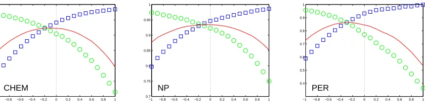
Figure 5 plots precision, recall and f-measure against the threshold for the basic multilabel model on the chemical substance, NP chunking and person entity extraction data sets. These plots clearly show what is expected: higher thresholds give higher pre-cision, and lower thresholds give higher recall. In these data sets at least, a zero threshold is almost always near optimal, though sometimes we would benefit from a slightly lower threshold.
5 Discussion
We have presented a method for text segmentation that is base on discriminatively learning structured multilabel classifications. The benefits include
• Competitive performance with sequential tag-ging models.
• Flexible modeling of complex segmentations, including overlapping, embedded and non-contiguous segments.
• Adjustable precision-recall trade off.
However, there is a computation cost for our models. For a text of length n, training and testing require
O(n3T) time, where T is the number of segment types. Fortunately, this still results in training times on the order of hours.
Our approach is related to the work of Bockhorst and Craven (2004). In this work, a conditional ran-dom field model is trained to allow for overlapping segments with an O(n2) inference algorithm. The model is applied to biological sequence modeling with promising results. However, our approaches differ in two major respects. First, their model is probabilistic, and trained to maximize segmenta-tion likelihood, while our model is trained to max-imize margin. Second, our method allows for non-contiguous segments, at the cost of a slowerO(n3)
inference algorithm.
In further work, the classification threshold should also be learned to achieve the desired balance between precision and recall. It would also be useful to investigate methods for combining these models with standard sequential tagging models to get top performance on simple segmentations as well as on overlapping or non-contiguous ones.
−1 −0.8 −0.6 −0.4 −0.2 0 0.2 0.4 0.6 0.8 1 0.4
0.5 0.6 0.7 0.8 0.9 1
CHEM
−1 −0.8 −0.6 −0.4 −0.2 0 0.2 0.4 0.6 0.8 1 0.7
0.75 0.8 0.85 0.9 0.95 1
NP
−1 −0.8 −0.6 −0.4 −0.2 0 0.2 0.4 0.6 0.8 1 0.4
0.5 0.6 0.7 0.8 0.9 1
[image:8.612.96.526.59.167.2]PER
Figure 5: Precision (squares), Recall (circles) and F-measure (line) plotted against threshold values. CHEM: chemical substance extraction, NP: noun-phrase chunking, and PER: person name extraction.
Acknowledgments
We thank the members of the Penn BioIE project for the development of the CYP450 corpus that we used for our experiments. In particular, Seth Kulick answered many questions about the data. This work has been supported by the NSF ITR grant 0205448.
References
D.M. Bikel, R. Schwartz, and R.M. Weischedel. 1999. An algorithm that learns what’s in a name. Machine
Learning Journal Special Issue on Natural Language Learning, 34(1/3):221–231.
J. Bockhorst and M. Craven. 2004. Markov networks for detecting overlapping elements in sequence data. In
Proc. NIPS.
Y. Censor and S.A. Zenios. 1997. Parallel optimization :
theory, algorithms, and applications. Oxford
Univer-sity Press.
M. Collins. 2002. Discriminative training methods for hidden Markov models: Theory and experiments with perceptron algorithms. In Proc. EMNLP.
K. Crammer and Y. Singer. 2002. A new family of online algorithms for category ranking. In Proc SIGIR.
K. Crammer. 2005. Online Learning for Complex
Cat-egorial Problems. Ph.D. thesis, Hebrew University of
Jerusalem. to appear.
N. Cristianini and J. Shawe-Taylor. 2000. An
Introduc-tion to Support Vector Machines. Cambridge
Univer-sity Press.
M. Dickinson and W.D. Meurers. 2005. Detecting errors in discontinuous structural annotation. In Proc. ACL.
A. Elisseeff and J. Weston. 2001. A kernel method for multi-labeled classification. In Proc. NIPS.
T. Kudo and Y. Matsumoto. 2001. Chunking with sup-port vector machines. In Proc. NAACL.
J. Lafferty, A. McCallum, and F. Pereira. 2001. Con-ditional random fields: Probabilistic models for seg-menting and labeling sequence data. In Proc. ICML.
A. McCallum, D. Freitag, and F. Pereira. 2000. Maxi-mum entropy Markov models for information extrac-tion and segmentaextrac-tion. In Proceedings of ICML.
R. McDonald, K. Crammer, and F. Pereira. 2004. Large margin online learning algorithms for scalable struc-tured classication. In NIPS Workshop on Strucstruc-tured
Outputs.
PennBioIE. 2005. Mining The Bibliome Project. http://bioie.ldc.upenn.edu/.
L. R. Rabiner. 1989. A tutorial on hidden Markov mod-els and selected applications in speech recognition.
Proceedings of the IEEE, 77(2):257–285, February.
A. Ratnaparkhi. 1996. A maximum entropy model for part-of-speech tagging. In Proc. EMNLP.
R. E. Schapire and Y. Singer. 1999. Improved boosting algorithms using confidence-rated predictions. Ma-chine Learning, 37(3):1–40.
B. Sch¨olkopf and A. J. Smola. 2002. Learning with
Ker-nels: Support Vector Machines, Regularization, Opti-mization and Beyond. MIT Press.
F. Sha and F. Pereira. 2003. Shallow parsing with condi-tional random fields. In Proc. HLT-NAACL.
B. Taskar, C. Guestrin, and D. Koller. 2003. Max-margin Markov networks. In Proc. NIPS.
E. F. Tjong Kim Sang and F. De Meulder. 2003. Intro-duction to the CoNLL-2003 shared task: Language-independent named entity recognition. In Proceedings
of CoNLL-2003.