Multi-loop PI/PID Controller Design Based on Direct Synthesis for Multivariable Systems

(1)

Multi-loop PI/PID Controller Design Based on

Direct Synthesis for Multivariable Systems

Abstract—In this paper, a new analytical method based on the direct synthesis approach is proposed for the design of a multi-loop proportional-integral-derivative (PID) controller. The proposed design method is aimed to achieve a desired closed-loop response for the multiple-input, multiple-output (MIMO) processes with multiple time delays. The ideal multi-loop controller is firstly designed in terms of relative gain and desired closed-loop transfer function. Then the standard multi-loop PID controller is obtained by approximating the ideal multi-loop controller by the Macraulin series expansion. Simulation study demonstrates the effectiveness of the proposed method the in multi-loop PID controller design. The multi-loop PID controller designed by the proposed method shows a fast, well-balanced, and robust response with the minimum integral absolute error (IAE).

Index Terms—Multi-loop PI/PID controller, Direct synthesis, Multivariable system. IMC-PID tuning, Robust controller design.

I. INTRODUCTION

The multi-loop PI/PID controllers, sometimes called as decentralized PI/PID controllers, have been widely utilized for processes with modest interactions for many decades because of many practical advantages such as a simple control structure, fewer tuning parameters, robustness against sensor/actuator failure, and easy understanding. Hence, many multi-loop design methods have been reported in the process control literature. However, most of the existing design methods are based on the extension of single-input, single-output (SISO) PI/PID controller design methods.

The modification of the Ziegler-Nichols (Z-N) method [1] with a detuning factor to meet the stability and performance of the multi-loop control system is a typical one of this class. In the family of the modified Ziegler-Nichols method [2]-[4], the desired critical point has to be determined by identifying the critical gain and frequency and then the multi-loop controllers are tuned by the Z-N tuning method with a weighting factor. However, a common disadvantage in these methods is that they try to cope with the interaction effect by detuning while neither dynamic nor static interactions is

incorporated in the design stage.

Another widely used approach is the extension of single-loop relay tuning to MIMO case [5],[6]. This approach is straightforward because it directly combines a single-loop relay auto-tuning and a sequential tuning, wherein the multi-loop control system is tuned sequentially loop by loop, closing the ith loop while it is tuned and the jth loop has to open [5]. However, the poor output responses can be obtained when the MIMO system has large multiple time delays which is one of main causes for the strong dynamic interactions.

It is well known that the integral model control (IMC) method [7] is very effective to design the IMC-PID controller for taking into account time delays and closed-loop interactions. Recently, several methods [8], [9] which extend the IMC-PID method of the SISO case to the MIMO case, are reported.

In this paper, a simple but efficient design method for multi-loop PI/PID controller is presented which exploits process interactions for the improvement of loop performance. The proposed method is based on the direct synthesis approach [10],[11] in which the multi-loop PI/PID controller is designed based on the desired closed-loop transfer function [8],[9],[12]. The resulting analytical design rule includes a frequency-dependent relative gain array [13], [14] that provides information of dynamic interactions useful for estimating the controller parameters.

Manuscript received July 22nd, 2008. This work was supported by Brain Korea (BK) 21.

Truong Nguyen Luan Vu and Moonyong Lee are with the School of Display & Chemical Engineering, Yeungnam University, 214-1, Dae-dong, Gyeongsan , Gyeongbuk 712-749, Korea (corresponding author to provide phone: 082-53-810-3241; fax: 082-53-811-3262; e-mails: [email protected], [email protected] ).

Truong Nguyen Luan Vu and Moonyong Lee

Gcn(s)

Gc2(s)

Gc1(s)

G(s)

Y1

R1

-Y2

R2

+

-Yn

Rn

+

(2)

II. MULTI-LOOP PI/PID CONTROLLER DESIGN A. The multi-loop feedback controller design for desired set-point responses

Consider a general transfer function matrix for stable, square, and multi-delays MIMO processes represented as following matrix:

11 12 1

21 22 2

1 2

( ) ( ) ( )

(s) =

( ) ( ) ( )

n n

n n nn

g s g s g s

g s g s g s

⎡ ⎤

⎢ ⎥

⎢ ⎢

⎢ ⎥

⎣ ⎦

G ⎥

⎥

(1)

From a standard block diagram of multi-loop feedback control shown in Fig. 1, the closed-loop transfer function matrix can be written as

(

)

1

( )s = ( )s _c( )s + ( )s _c( )s −

H G G I G G (2)

Consider a transfer function H( )s of a diagonal structure for a desired closed-loop response. Then the feedback controller to give the desired closed-loop response can be straightforwardly found by rearranging (2). However, the resulting controller is generally not a diagonal (or decentralized) form. By taking off all off-diagonal elements from the resulting centralized controller, one can obtain a multi-loop (or decentralized) feedback controller as follows:

{

1

}

( ) ( ) ( ) ( )

C s diag s s s

−

⎡ ⎤

= _⎣ − _⎦

-1

G G H I H (3)

It is clear that the controller by (3) gives a closed-loop response closer to the desired one as process interactions are insignificant. Since the multi-loop controllers are usually applied to processes with modest interactions, this approach can have validity.

Note that the multi-loop controller by (3) is not a standard PID form. The controller above consists of two parts. i.e.,

1

( )s −

G and H( )s ⎡_⎣I − H( )s ⎤_⎦−1.

1

( )s −

G can be written as

1 (s)

( )

(s) adj s

− ₌ G

G

(4)

where adjG = ⎣⎡Gji⎤⎦ and is the cofactor corresponding to in G ;

ij

G

ij

g

G

( )

s

denotes the determinant of

G

( )

s

.

Furthermore, can be expressed in

terms of diagonal element as

1

( )

s

⎡ −

_⎣

( )

s

−

H

I

H

⎤⎦

1 1

( )

1 ( )

-1 ii

ii

h s

s

diag

h s

− −

⎡

⎤

⎡

−

⎤

=

⎡

−

⎤

=

_⎢

_⎥

⎣

⎦

⎣

⎦

_⎣

₋

_⎦

H

I H

H

I

(5)

where

h

_ii is each diagonal element of H( )s and corresponds to the desired servo closed-loop transfer function for each loop.

Substituting (4) and (5) into (3) gives

( )

1 ( )

ii C

ii

h s

adj

s

diag

s

h s

⎧

⎡

⎤

⎫

⎪

=

_⎨

_{⎢ −}

_⎥

_⎬

⎪

⎣

⎦

⎪

⎩

⎭

G

(6)

Therefore, each element of the multi-loop controller can be derived as

( )

(s)

1 ( )

ii

ii ci

ii

h s

s

g s

h s

⎛

⎞

=

_{⎜ −}

⎝

⎠

G

⎟

(7)

From Bristol [14], the diagonal element of the frequency-dependent relative gain array for G(s) is calculated by

( )

ii ii ii

s

g s

s

Λ

=

G

(8)

Hence, by substituting (8) into (7), each element of the multi-loop controller can be obtained as

1

( )

1 ( )

ii ci ii ii

ii

h s

g s

s g

s

h s

−

⎛

⎞

= Λ

_{⎜ −}

⎝

⎠

⎟

(9)

According to the IMC theory [7], the desired closed-loop transfer function

h s

_ii

( )

is chosen as

* 1

( )

,

1, 2,

,

i

ii

q

s k

ii i

k k

s z

h s

e

f s

i

n

s z

θ −

=

− +

=

+

∏

…

(10)

where

z

k,

*

k

z

and

θ

ii denote the right-haft-plane (RHP)

zeros of the (i, i)th diagonal element of the process transfer function matrix, the corresponding complex conjugate of RHP zeros, and the time delay term, respectively; denotes the number of ;

i

q

k

z

f s

_i

( )

is the IMC filter of the ith loop and chosen simply as

(

)

1 ( )

1

i

i r

i

f s

s

λ

=

+

(11)

The IMC filter time constant

λ

_i, which is also equivalent to the closed-loop time constant, is an adjustable parameter to achieve the adequate tradeoff between performance and robustness.

(3)

(

)

* 1 1 * 1

( )

1

i ii i i _ii q s k k k

ci ii ii q

r _s _k i

k k

z

s

e

z

s

g s

s g s

z

s

e

z

s

θ θ

λ

− − = − =

⎛

−

⎞

⎜

₊

⎟

⎜

⎟

= Λ

⎜

₊

₋

−

⎟

⎜

₊

⎟

⎝

⎠

∏

(12)

Note that in (12), the non-minimum portion of is cancelled out with the time delay and RHP zero z

( )

ii

g s

k in the

numerator so that the controller has neither causality nor stability problem.

B. Reduction to the multi-loop PI/PID controller

For processes with multi-delays, the proposed multi-loop controller can be found by the following procedure:

n x n

The multi-loop feedback controller can be rewritten as

1

( )

ci ii

g s

≡

s p s

− (13)

Thus,

(

)

* 1 1 * 1

( )

1

i ii i i _ii q s k k k

ii ii ii q

r _s _k i

k k

z s

e

z s

p s

s

s g s

z s

s

e

z s

θ θ

λ

− − = − =

⎛

−

⎜

₊

⎟

⎜

⎟

≡ Λ

⎜

₊

₋

−

⎜

₊

⎝

⎠

∏

⎞

⎟

(14)

Furthermore, (13) can be expanded by using the Maclaurin series as

2

(0)

1 ( )

(0)

2

ii ci ii ii

p

g s

p

sp

s

′′

⎡

_′

⎤

=

_⎢

+

_⎥

⎣

…

⎦

(15)

Since the standard form of multi-loop PID controller is given by

2

1 ( )

Ci s = _s⎡⎣ Ii+s Ci+s Di⎤⎦

G K K K (16)

The proposed PID controller is found by the comparison between (15) and (16).

{

(0)

}

Ci

=

diag p

ii

′

K

(17)

{

(0)

}

Ii

=

diag p

ii

K

(18)

{

(0) / 2

}

Di

=

diag p

ii

′′

K

(19)

From (17), (18), and (19), it is straightforward to design the multi-loop PI/PID controller for various multivariable processes with delays.

C. Example of two-input, two-output (TITO) case

The TITO multi-delay processes are very popular in the process industry. In this section, the TITO multi-delay processes with the first-order plus delay time (FOPDT) dynamics are considered. The multi-loop feedback controller can be obtained from (12) as

(

)

(

)

1

1 ( )

( )

1

ii ii

ci ii s

ii i

T s

g s

s

K

λ

s

e

−θ

⎛

⎞

+

= Λ

⎜

_⎜

⎟

_⎟

+ −

⎝

⎠

(20)

where and denote the gain and time constant of , respectively. The order of the IMC filter is selected as 1 for the controller to be realizable.

ii

K

T

_ii

g

_ii

The (i, i)th element of the frequency-dependent relative gain array is calculated by

(

)(

)

(

11

)(

22

)

12 21

11 22 12 21

1 ( )

1

ei ii s

s

T s

K K

e

K K

T s

θ −

Λ

=

+

−

+

(21)

where the effective delay

θ

ei is defined by

12 21 11 22

ei

θ

=

θ

+

θ

−

θ

−

θ

.

Substituting (21) into (20), an analytical tuning rule of the multi-loop PI controller can be obtained by using (17) and (18) as

( )(

)

(

)

{

}

2 2 (0)

2 ( )

2 0

ii Ci

ii i ii

ii ii i ii ei ei ei ii

K

K T T

λ θ

θ

λ θ

θ

Λ

= ×

+

+ Λ + ⎡_⎣ − + ⎤_⎦

K (22)

(0)

(

)

ii Ii

ii i ii

K

λ θ

Λ

=

+

K

(23)

where

K

_ei denotes the interaction quotient [15] and

12 21 11 22 ei

K K

K

K K

=

. The effective time constant is defined

as

ei

T

,

ci jj ij ji

T

=

T

− −

T

j i

≠

. It is noted that

Λ

ii

(0)

corresponds to the diagonal

element of the steady-state relative gain array (RGA) by Bristol [14].

III. ROBUST STABILITY ANALYSIS

(4)

uncertainty, which cause a poor performance or even instability in control systems. In this study, the well known robustness analysis [16], [17] is introduced for fair comparison with other existing controller design methods.

The robust stability can be examined under the output multiplication uncertainty. For the multi-delay process with the output multiplicative uncertainty of , the upper bound of robust stability can be written by

0

∆

( )

{

(

)

}

(

)

1 0

1

1/

( ) ( )

,

0

c c

c

I

j

I

j

γ σ

σ

ω

σ

ω

−

⎡

= ∆ <

_⎢⎣

+

⎡

⎤

<

_⎢

+

_⎥

∀ ≥

⎣

⎦

G

⎤

⎥⎦

)

(24)

where

G

(

j

ω

)

G

c

(

j

ω

is invertible.

For fair comparison, the degree of robust stability will be hold at the same level for all design methods compared. In the simulation study, the proposed multi-loop PI/PID controller is tuned by adjusting the closed-loop time constant

λ

_iso that the

γ

value of the proposed control system should be kept as same as or at least larger than those by the other comparative methods.

(a)

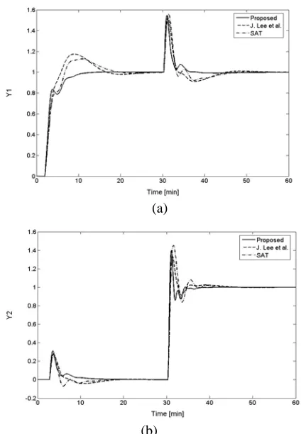
[image:4.595.61.273.374.680.2]

(b)

Fig. 2 Closed-loop responses for VL column by sequential set-point changes in loop 1 and loop 2.

IV. SIMULATIONSTUDY

Example 1: Consider the following Vinante and Luyben (VL) column studied by W. Luyben [3].

- s -0.3 s

-1.8 s -0.35 s

-2.2 e

1.3 e

7s + 1

G(s)=

-2.8e

4.3e

9.5s + 1

9.2s + 1

⎡

⎤

⎢

⎥

⎢

⎥

⎢

⎥

⎢

⎥

⎣

⎦

(25)

[image:4.595.314.548.486.582.2]

In this example,

γ

is chosen as 0.53 both for the proposed and J. Lee [16] design methods. From (24),

λ

_iare obtained as 1.55 and 0.25 for loop 1 and loop 2, respectively. All control parameters are listed in Table I. Fig. 2 shows that the proposed method provides a stable and robust response. As shown in Table I, the proposed design method gives the best closed-loop performance in terms of IAE under the same or more robust stability.

Table I: Controller parameters and performance indices by the various methods: VL column

Proposed J. Lee SAT Kc _{-1.9, 5.45} _{-1.31, 3.97} _{-1.35, 3.36}

I

τ _{6.54, 8.65} _{2.26, 2.42} _{3.00, 1.33}

IAEt 5.68 7.19 7.28

γ

_{0.53 0.53 0.40}

IAEt : total sum of IAE of each loop.

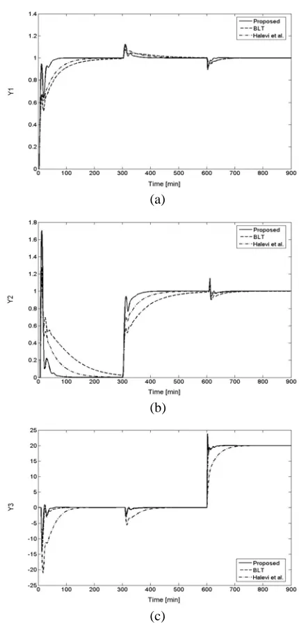
Example 2. A multi-product distillation column for separation of binary ethanol-water mixture was modeled experimentally [18]. The transfer function matrix of the OR column is given by

2.6 3.5

6.5 3 12

9.2 9.4

0.66 0.6 0.0049

6.7 1 8.64 1 9.06 1

1.11 2.36 0.01

( )

3.25 1 5 1 7.09 1

34.68 46.2 0.89(11.61 1)

8.15 1 10.9 1 (3.89 1)(18.8 1)

s s s

s s

e e e

s s s

e e e

G s

s s s

e e s e

s s s s

− − −

− − −s

⎡ − − ⎤

⎢ ₊ ₊ ₊ ⎥

⎢ ⎥

− −

⎢ ⎥

= ⎢ ₊ ₊ ₊ ⎥

⎢ ⎥

− +

⎢ ⎥

⎢ ₊ ₊ ₊ ₊ ⎥

⎣ ⎦

(26)

For a fair comparison, the upper bound

γ

of robust stability of the proposed method is selected by 0.035 same as those by the BLT [3] and Y. Halevi [6] methods. Accordingly, the closed-loop time constant

λ

_i is found as 8.85, 8.85, and 1.65 for loop 1, 2, and 3, respectively.

(5)

(a)

(b)

[image:5.595.60.275.51.502.2]

(c)

Fig. 3 Closed-loop responses for OR column by sequential set-point changes in loop 1, 2 and 3.

Table II: Controller parameters and performance indices by the various methods: OR column

The IAE values listed in Table II also show the superiority of the proposed method over the other existing methods.

V. CONCLUSIONS

In this paper, a novel analytical design method is proposed for the multi-delay processes. The proposed method is straightforward and easy to implement on the multi-loop control systems. The robust stability and performance can be efficiently fixed by adjusting a single parameter, i.e., the closed-loop time constant.

The time-domain simulation illustrates that the proposed control system provides a fast and well-balanced closed-loop time responses.

REFERENCES

[1] J. G. Ziegler, N. B. Nichols, “Optimum settings for automatic controllers,” Trans. ASME , vol. 64, 1942, pp.759-768.

[2] A. Niederlinski, “A heuristic approach to the design of linear multivariable interacting control systems,” Automatica, vol. 7, 1971, pp. 691-701.

[3] W. L. Luyben, “Simple method for tuning SISO controllers in multivariable systems,” Ind. Eng. Chem. Process Des. Dev., vol. 25, 1986, pp. 654-660.

[4] J. Lee, T. F. Edgar, “Continuation method for the modified Ziegler - Nichols tuning of multi-loop control systems,” Ind. Eng. Chem.Res, vol. 44, 2005, pp. 7428-7434.

[5] A. P. Loh, C. C. Hang, C. K. Quek, and V. U. Vasnani, “Autotuning of multi-loop proportional - integral controllers using relay feedback,” In. Eng. Chem. Res., , vol. 32, 1993, pp. 1102-1107. [6] Y. Halevi, Z. J. Palmor, and T. Efrati, “Automatic tuning of

decentralized PID controllers for MIMO processes,” Journal of Process Control, vol. 7, 1997, pp. 119-128.

[7] M. Morari., E. Zafiriou, Robust process control, New Jersey:Prentice Hall-Englewood Cliffs, 1989, ch. 4.

[8] M. Lee, K. Lee, C. Kim, and J. Lee, “Analytical design of multi-loop PID controllers for desired closed-loop responses,” AIChE , vol.50, 2004, pp. 1631-165.

[9] L. V. Truong-Nguyen, J. Lee, M. Lee, “Design of multi-loop PID controllers based on the generalized IMC-PID method with Mp criterion,” IJCAS, vol.5, 2007, pp. 212-218.

[10] J. G. Truxal, Automatic Feedback Control System Synthesis, New York: McGraw-Hill, 1955.

[11] D. E. Seborg, T. F. Edgar, D. A. Mellichamp, Process Dynamics and Control, New York: John Wiley & Sons. 1989.

[12] Q.G. Wang, T. H. Lee, C. Lin., Relay feedback: analysis, identification and control, London : Springer, 2003.

[13] S. Skogestad, I. Postlethwaithe, Multivariable feedback control analysis and design, New York: John Wiley & Sons, 2005.

[14] E. H. Bristol, “Recent results on interactions in multivariable process control,” Proceedings of the 71st annual AIChE meeting, Houston, USA, 1979.

[15] J.E Rijnsdorp, “Interaction in two-variable control system for distillation columns-I and II,” Automatica, vol. 1, 1965, pp. 15-28. [16] J. Lee, W. Cho, T. F. Edgar, “Multi-loop PI controller tuning for

interacting multivariable processes,” Comp. Chem. Eng., vol.22, 1998, pp.1711-1723.

Proposed BLT Y. Halevi Kc 1.567

-0.310 6.102

1.510 -0.295 2.630

1.250 -0.339 0.923 I

τ 5.956

4.811 9.596

16.40 18.00 6.610

10.50 10.50 10.50

IAEt 184.676 363.503 979.124

γ

_{0.035 0.035 0.035}

[17] S. L. William, Control system fundamentals, Florida: CRC Press LLC, 1999.

[image:5.595.56.279.585.712.2]