Proceedings of the 2011 Conference on Empirical Methods in Natural Language Processing, pages 38–49,
Optimal Search for Minimum Error Rate Training
Michel Galley Microsoft Research Redmond, WA 98052, USA [email protected]
Chris Quirk Microsoft Research Redmond, WA 98052, USA [email protected]
Abstract
Minimum error rate training is a crucial compo-nent to many state-of-the-art NLP applications, such as machine translation and speech recog-nition. However, common evaluation functions such as BLEU or word error rate are generally highly non-convex and thus prone to search errors. In this paper, we present LP-MERT, an exact search algorithm for minimum error rate training that reaches the global optimum using a series of reductions to linear programming. Given a set ofN-best lists produced fromS input sentences, this algorithm finds a linear model that is globally optimal with respect to this set. We find that this algorithm is poly-nomial inNand in the size of the model, but exponential inS. We present extensions of this work that let us scale to reasonably large tuning sets (e.g., one thousand sentences), by either searching only promising regions of the param-eter space, or by using a variant of LP-MERT that relies on a beam-search approximation. Experimental results show improvements over the standard Och algorithm.
1 Introduction
Minimum error rate training (MERT)—also known as direct loss minimization in machine learning—is a crucial component in many complex natural language applications such as speech recognition (Chou et al., 1993; Stolcke et al., 1997; Juang et al., 1997), statisti-cal machine translation (Och, 2003; Smith and Eisner, 2006; Duh and Kirchhoff, 2008; Chiang et al., 2008), dependency parsing (McDonald et al., 2005), summa-rization (McDonald, 2006), and phonetic alignment (McAllester et al., 2010). MERT directly optimizes the evaluation metric under which systems are being evaluated, yielding superior performance (Och, 2003) when compared to a likelihood-based discriminative
method (Och and Ney, 2002). In complex text gener-ation tasks like SMT, the ability to optimize BLEU (Papineni et al., 2001), TER (Snover et al., 2006), and other evaluation metrics is critical, since these met-rics measure qualities (such as fluency and adequacy) that often do not correlate well with task-agnostic loss functions such as log-loss.
While competitive in practice, MERT faces several challenges, the most significant of which is search. The unsmoothed error count is a highly non-convex objective function and therefore difficult to optimize directly; prior work offers no algorithm with a good approximation guarantee. While much of the ear-lier work in MERT (Chou et al., 1993; Juang et al., 1997) relies on standard convex optimization tech-niques applied to non-convex problems, the Och al-gorithm (Och, 2003) represents a significant advance for MERT since it applies a series of special line min-imizations that happen to be exhaustive and efficient. Since this algorithm remains inexact in the multidi-mensional case, much of the recent work on MERT has focused on extending Och’s algorithm to find better search directions and starting points (Cer et al., 2008; Moore and Quirk, 2008), and on experiment-ing with other derivative-free methods such as the Nelder-Mead simplex algorithm (Nelder and Mead, 1965; Zens et al., 2007; Zhao and Chen, 2009).
In this paper, we present LP-MERT, an exact search algorithm for N-best optimization that
ex-ploits general assumptions commonly made with MERT, e.g., that the error metric is decomposable by sentence.1 While there is no known optimal
algo-1Note that MERT makes two types of approximations. First,
the set of all possible outputs is represented only approximately, byN-best lists, lattices, or hypergraphs. Second, error
rithm to optimize general non-convex functions, the unsmoothed error surface has a special property that enables exact search: the set of translations produced by an SMT system for a given input is finite, so the piecewise-constant error surface contains only a fi-nitenumber of constant regions. As in Och (2003), one could imagine exhaustively enumerating all con-stant regions and finally return the best scoring one— Och does this efficiently with each one-dimensional search—but the idea doesn’t quite scale when search-ing all dimensions at once. Instead, LP-MERT ex-ploits algorithmic devices such as lazy enumeration, divide-and-conquer, and linear programming to effi-ciently discard partial solutions that cannot be max-imized by any linear model. Our experiments with thousands of searches show that LP-MERT is never worse than the Och algorithm, which provides strong evidence that our algorithm is indeed exact. In the appendix, we formally prove that this search algo-rithm is optimal. We show that this algoalgo-rithm is polynomial inN and in the size of the model, but
exponential in the number of tuning sentences. To handle reasonably large tuning sets, we present two modifications of LP-MERT that either search only promising regions of the parameter space, or that rely on a beam-search approximation. The latter modifica-tion copes with tuning sets of one thousand sentences or more, and outperforms the Och algorithm on a WMT 2010 evaluation task.
This paper makes the following contributions. To our knowledge, it is the first known exact search algorithm for optimizing task loss onN-best lists in general dimensions. We also present an approximate version of LP-MERT that offers a natural means of trading speed for accuracy, as we are guaranteed to eventually find the global optimum as we gradually increase beam size. This trade-off may be beneficial in commercial settings and in large-scale evaluations like the NIST evaluation, i.e., when one has a stable system and is willing to let MERT run for days or weeks to get the best possible accuracy. We think this work would also be useful as we turn to more human involvement in training (Zaidan and Callison-Burch, 2009), as MERT in this case is intrinsically slow.
2 Unidimensional MERT
Let fS1 = f1. . .fS denote the S input sentences of our tuning set. For each sentencefs, letCs =
es,1. . .es,N denote a set ofNcandidate translations. For simplicity and without loss of generality, we assume thatN is constant for each index s. Each input and output sentence pair(fs,es,n)is weighted by a linear model that combines model parameters
w = w1. . . wD ∈ RD with D feature functions
h1(f,e,∼). . . hD(f,e,∼), where ∼ is the hidden state associated with the derivation fromf toe, such
as phrase segmentation and alignment. Furthermore, leths,n∈RD denote the feature vector representing the translation pair(fs,es,n).
In MERT, the goal is to minimize an error count
E(r,e)by scoring translation hypotheses against a
set of reference translations rS1 = r1. . .rS.
As-suming as in Och (2003) that error count is addi-tively decomposable by sentence—i.e.,E(rS1,eS1) = P
sE(rs,es)—this results in the following optimiza-tion problem:2
ˆ
w= arg min w
XS
s=1
E(rs,ˆe(fs;w))
= arg min w
XS
s=1
N X
n=1
E(rs,es,n)δ(es,n,ˆe(fs;w))
(1) where
ˆ
e(fs;w) = arg max n∈{1...N}
w|hs,n
The quality of this approximation is dependent on how accurately theN-best lists represent the search
space of the system. Therefore, the hypothesis list is iteratively grown: decoding with an initial parameter vector seeds theN-best lists; next, parameter esti-mation andN-best list gathering alternate until the
search space is deemed representative.
The crucial observation of Och (2003) is that the error count along any line is a piecewise constant function. Furthermore, this function for a single sen-tence may be computed efficiently by first finding the hypotheses that form the upper envelope of the model score function, then gathering the error count for each hypothesis along the range for which it is optimal. Er-ror counts for the whole corpus are simply the sums of these piecewise constant functions, leading to an
2A metric such as TER is decomposable by sentence. BLEU
efficient algorithm for finding the global optimum of the error count along any single direction.
Such a hill-climbing algorithm in a non-convex space has no optimality guarantee: without a perfect direction finder, even a globally-exact line search may never encounter the global optimum. Coordinate as-cent is often effective, though conjugate direction set finding algorithms, such as Powell’s method (Powell, 1964; Press et al., 2007), or even random directions may produce better results (Cer et al., 2008). Ran-dom restarts, based on either uniform sampling or a random walk (Moore and Quirk, 2008), increase the likelihood of finding a good solution. Since random restarts and random walks lead to better solutions and faster convergence, we incorporate them into our baseline system, which we refer to as 1D-MERT.
3 Multidimensional MERT
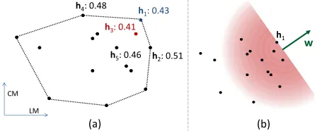
Finding the global optimum of Eq. 1 is a difficult task, so we proceed in steps and first analyze the case where the tuning set contains only one sentence. This gives insight on how to solve the general case. With only one sentence, one of the two summations in Eq. 1 vanishes and one can exhaustively enumer-ate theN translationse1,n (oren for short) to find the one that yields the minimal task loss. The only difficulty withS= 1is to know for each translation enwhether its feature vectorh1,n (orhnfor short) can be maximized using any linear model. As we can see in Fig. 1(a), some hypotheses can be maxi-mized (e.g.,h1,h2, andh4), while others (e.g.,h3
andh5) cannot. In geometric terminology, the former
points are commonly calledextremepoints, and the latter areinteriorpoints.3 The problem of exactly
optimizing a singleN-best list is closely related to
the convex hull problem in computational geometry, for which generic solvers such as the QuickHull al-gorithm exist (Eddy, 1977; Bykat, 1978; Barber et al., 1996). A first approach would be to construct the convex hullconv(h1. . .hN)of theN-best list, then identify the point on the hull with lowest loss (h1in
Fig. 1) and finally compute an optimal weight vector using hull points that share common facets with the
3Specifically, a pointhis extreme with respect to a convex
setC(e.g., the convex hull shown in Fig. 1(a)) if it does not lie in an open line segment joining any two points ofC. In a minor abuse of terminology, we sometimes simply state that a given pointhis extreme when the nature ofCis clear from context.
w
h1
h3:0.41
h1: 0.43
h4: 0.48
h5: 0.46 h2: 0.51
LM CM
[image:3.612.315.539.72.165.2](a) (b)
Figure 1:N-best list(h1. . .hN)with associated losses
(here, TER scores) for a single input sentence, whose convex hull is displayed with dotted lines in (a). For effec-tive visualization, our plots use only two features (D= 2). While we can find a weight vector that maximizesh1(e.g.,
thewin (b)), no linear model can possibly maximize any of the points strictly inside the convex hull.
optimal feature vector (h2 andh4). Unfortunately,
this doesn’t quite scale even with a singleN-best list,
since the best known convex hull algorithm runs in
O(NbD/2c+1)time (Barber et al., 1996).4
Algorithms presented in this paper assume thatD
is unrestricted, therefore we cannot afford to build any convex hull explicitly. Thus, we turn to linear programming (LP), for which we know algorithms (Karmarkar, 1984) that are polynomial in the number of dimensions and linear in the number of points, i.e.,
O(N T), whereT = D3.5. To check if pointhi is extreme, we really only need to know whether we can define a half-space containing all pointsh1. . .hN, withhilying on the hyperplane delimiting that half-space, as shown in Fig. 1(b) for h1. Formally, a
vertexhiis optimal with respect toarg maxi{w|hi} if and only if the following constraints hold:5
w|hi =y (2)
w|hj ≤y, for each j6=i (3)
wis orthogonal to the hyperplane defining the half-space, and the interceptydefines its position. The
4A convex hull algorithm polynomial inDis very unlikely.
Indeed, the expected number of facets of high-dimensional con-vex hulls grows dramatically, and—assuming a uniform distribu-tion of points,D= 10, and a sufficiently largeN—the expected
number of facets is approximately106N(Buchta et al., 1985).
In the worst case, the maximum number of facets of a convex hull isO(NbD/2c/bD/2c!)(Klee, 1966).
5A similar approach for checking whether a given point is
extreme is presented inhttp://www.ifor.math.ethz.
ch/˜fukuda/polyfaq/node22.html, but our method
above equations represent a linear program (LP), which can be turned into canonical form
maximize c|w
subject to Aw≤b
by substituting y withw|hi in Eq. 3, by defining
A = {an,d}1≤n≤N;1≤d≤D withan,d = hj,d−hi,d
(wherehj,dis thed-th element ofhj), and by setting
b = (0, . . . ,0)| = 0. The vertexhi is extreme if and only if the LP solver finds a non-zero vectorw
satisfying the canonical system. To ensure thatwis zero only whenhi is interior, we setc = hi−hµ, wherehµis a point known to be inside the hull (e.g., the centroid of theN-best list).6 In the remaining
of this section, we use this LP formulation in func-tion LINOPTIMIZER(hi;h1. . .hN), which returns the weight vectorwˆ maximizinghi, or which returns 0ifhi is interior toconv(h1. . .hN). We also use
conv(hi;h1. . .hN)to denote whetherhiis extreme with respect to this hull.
Algorithm 1:LP-MERT (forS= 1).
input :sent.-level feature vectorsH ={h1. . .hN}
input :sent.-level task lossesE1. . . EN, where
En:=E(r1,e1,n)
output:optimal weight vectorwˆ
1 begin
.sortN-best list by increasing losses:
2 (i1. . . iN)←INDEXSORT(E1. . . EN)
3 forn←1toNdo
.findwˆ maximizingin-th element:
4 wˆ←LINOPTIMIZER(hin;H) 5 ifwˆ6=0then
6 returnwˆ
7 return0
An exact search algorithm for optimizing a single
N-best list is shown above. It lazily enumerates
fea-ture vectors in increasing order of task loss, keeping only the extreme ones. Such a vertexhj is known to be on the convex hull, and the returned vectorwˆ
max-imizes it. In Fig. 1, it would first run LINOPTIMIZER onh3, discard it since it is interior, and finally accept
the extreme pointh1. Each execution of
LINOPTI-MIZERrequiresO(N T)time with the interior point 6We assume thath
1. . .hNare not degenerate, i.e., that they collectively spanRD. Otherwise, all points are necessarily on the hull, yet some of them may not be uniquely maximized.
0.001 0.01 0.1 1 10 100 1000 10000 100000
2 3 4 5 6 7 8 9 10 11 12 13 14 15 16 17 18 19 20 QuickHull
LP
Dimensions
Sec
on
d
[image:4.612.317.536.73.231.2]s
Figure 2: Running times to exactly optimizeN-best lists with an increasing number of dimensions. To determine which feature vectors were on the hull, we use either linear programming (Karmarkar, 1984) or one of the most effi-cient convex hull computation tools (Barber et al., 1996).
method of (Karmarkar, 1984), and since the main loop may runO(N) times in the worst case, time
complexity isO(N2T). Finally, Fig. 2 empirically
demonstrates the effectiveness of a linear program-ming approach, which in practice is seldom affected byD.
3.1 Exact search: general case
We now extend LP-MERT to the general case, in which we are optimizing multiple sentences at once. This creates an intricate optimization problem, since the inner summations over n = 1. . . N in Eq. 1
can’t be optimized independently. For instance, the optimal weight vector for sentences = 1 may
be suboptimal with respect to sentence s = 2.
So we need some means to determine whether a selectionm = m(1). . . m(S)∈ M = [1, N]S of
feature vectorsh1,m(1). . .hS,m(S)is extreme, that is,
whether we can find a weight vector that maximizes eachhs,m(s). Here is a reformulation of Eq. 1 that
makes this condition on extremity more explicit:
ˆ
m= arg min
conv(h[m];H) m∈M
XS
s=1
E(rs,es,m(n))
(4)
where
h[m] =
S X
s=1
hs,m(s)
H= [
One na¨ıve approach to address this optimization problem is to enumerate all possible combinations among theSdistinctN-best lists, determine for each combinationmwhetherh[m]is extreme, and return
the extreme combination with lowest total loss. It is evident that this approach is optimal (since it follows directly from Eq. 4), but it is prohibitively slow since it processesO(NS) vertices to determine whether
they are extreme, which thus requiresO(NST)time
per LP optimization andO(N2ST)time in total. We now present several improvements to make this ap-proach more practical.
3.1.1 Sparse hypothesis combination
In the na¨ıve approach presented above, each LP computation to evaluate conv(h[m];H) requires O(NST) time since H contains NS vertices, but
we show here how to reduce it to O(N ST) time.
This improvement exploits the fact that we can elimi-nate the majority of theNSpoints ofH, since only
S(N−1) + 1are really needed to determine whether
h[m]is extreme. This is best illustrated using an
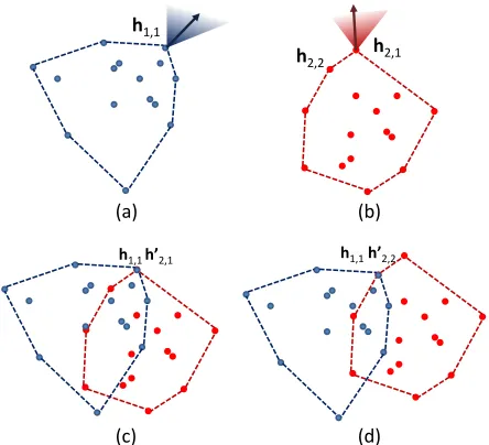
ex-ample, as shown in Fig. 3. Bothh1,1andh2,1in (a)
and (b) are extreme with respect to their ownN-best
list, and we ask whether we can find a weight vector that maximizes both h1,1 and h2,1. The
algorith-mic trick is to geometrically translate one of the two
N-best lists so thath1,1 = h20,1, where h02,1 is the
translation ofh02,1. Then we use linear programming with the new set of2N−1points, as shown in (c), to
determine whetherh1,1is on the hull, in which case
the answer to the original question is yes. In the case of the combination ofh1,1andh2,2, we see in (d) that
the combined set of points prevents the maximization
h1,1, since this point is clearly no longer on the hull.
Hence, the combination (h1,1,h2,2) cannot be
maxi-mized using any linear model. This trick generalizes toS ≥2. In both (c) and (d), we usedS(N −1) + 1
points instead ofNSto determine whether a given
point is extreme. We show in the appendix that this simplification does not sacrifice optimality.
3.1.2 Lazy enumeration, divide-and-conquer
Now that we can determine whether a given combi-nation is extreme, we must next enumerate candidate combinations to find the combination that has low-est task loss among all of those that are extreme. Since the number of feature vector combinations is
O(NS), exhaustive enumeration is not a reasonable
h1,1
h2,2 h2,1
(a) (b)
h1,1 h’2,2
(c) (d)
[image:5.612.316.538.72.274.2]h1,1 h’2,1
Figure 3: Given two N-best lists, (a) and (b), we use linear programming to determine which hypothesis com-binations are extreme. For instance, the combinationh1,1
andh2,1is extreme (c), whileh1,1andh2,2is not (d).
option. Instead, we use lazy enumeration to pro-cess combinations in increasing order of task loss, which ensures that the first extreme combination for
s= 1. . . Sthat we encounter is the optimal one. An S-ary lazy enumeration would not be particularly
ef-ficient, since the runtime is stillO(NS)in the worst case. LP-MERT instead uses divide-and-conquer and binary lazy enumeration, which enables us to discard early on combinations that are not extreme. For instance, if we find that (h1,1,h2,2) is interior for
sentencess= 1,2, the divide-and-conquer branch
fors= 1. . .4never actually receives this bad
com-bination from its left child, thus avoiding the cost of enumerating combinations that are known to be interior, e.g., (h1,1,h2,2,h3,1,h4,1).
The LP-MERT algorithm for the general case is shown as Algorithm 2. It basically only calls a re-cursive divide-and-conquer function (GETNEXTBEST)
for sentence range1. . . S. The latter function uses
bi-nary lazy enumeration in a manner similar to (Huang and Chiang, 2005), and relies on two global variables:
IandL. The first of these,I, is used to memoize the
results of calls to GETNEXTBEST; given a range of sentences and a rankn, it stores thenth best combina-tion for that range of sentences. The global variable
h11 h
12 h
21 h22 h23
69.1 69.2 69.3
69.2 69.4
h 31 h32 h
33 h
41 h42
56.8 57.1 57.3 57.6
h 23
57.9 {h
11, h23}
{h 31, h41}
126.0 126.5 126.1
{h 32, h41}
{h 12, h21}
Combinations checked:
{h
11, h23, h31, h41}
{h12, h21, h31, h41}
Combinations discarded:
{h
11, h21, h31, h41}
{h
12, h22, h31, h41}
{h12, h12, h31, h42} (and 7 others)
h13
h 24
69.9 70.0
L[3,4]
[image:6.612.73.295.72.162.2]L[1,2]
Figure 4: LP-MERT minimizes loss (TER) on four sen-tences. O(N4) translation combinations are possible,
but the LP-MERT algorithm only tests two full combi-nations. Without divide-and-conquer—i.e., using 4-ary lazy enumeration—ten full combinations would have been checked unnecessarily.
Algorithm 2:LP-MERT
input :feature vectorsH={hs,n}1≤s≤S;1≤n≤N
input :task lossesE={Es,n}1≤s≤S;1≤n≤N,
where sent.-level costsEs,n:=E(rs,es,n)
output:optimal weight vectorwˆand its lossL
1 begin
.sortN-best lists by increasing losses:
2 fors←1toSdo
3 (is,1..is,N)←INDEXSORT(Es,1..Es,N)
.find best hypothesis combination for1. . . S: 4 (h∗, H∗, L)←GETNEXTBEST(H,E,1, S) 5 wˆ←LINOPTIMIZER(h∗;H∗)
[image:6.612.309.545.80.517.2]6 return(ˆw, L)
Fig. 4, to determine which combination to try next. The function EXPANDFRONTIERreturns the indices
of unvisited cells that are adjacent (right or down) to visited cells and that might correspond to the next best hypothesis. Once no more cells need to be added to the frontier, LP-MERT identifies the lowest loss combination on the frontier (BESTINFRONTIER), and
uses LP to determine whether it is extreme. To do so, it first generates an LP using COMBINE, a function
that implements the method described in Fig. 3. If the LP offers no solution, this combination is ignored. LP-MERT iterates until it finds a cell entry whose combination is extreme. Regarding ranges of length one (s=t), lines 3-10 are similar to Algorithm 1 for S = 1, but with one difference:GETNEXTBESTmay
be called multiple times with the same arguments,
since the first output ofGETNEXTBESTmight not be
extreme when combined with other feature vectors. Lines 3-10 ofGETNEXTBEST handle this case
effi-ciently, since the algorithm resumes at the(n+ 1)-th
FunctionGetNextBest(H,E,s,t)
input :sentence range(s, t)
output:h∗: current best extreme vertex
output:H∗: constraint vertices
output:L: task loss ofh∗
.Losses of partial hypotheses:
1 L← L[s, t] 2 ifs=tthen
. nis the index where we left off last time:
3 n←NBROWS(L) 4 Hs← {hs,1. . .hs,N}
5 repeat
6 n←n+ 1
7 wˆ←LINOPTIMIZER(hs,in;Hs) 8 L[n,1]←Es,in
9 untilwˆ6=0
10 return(hs,in, Hs,L[n,1]) 11 else
12 u← b(s+t)/2c,v←u+ 1
13 repeat
14 whileHASINCOMPLETEFRONTIER(L)do
15 (m, n)←EXPANDFRONTIER(L)
16 x←NBROWS(L)
17 y←NBCOLUMNS(L)
18 form0←x+ 1tomdo
19 I[s, u, m0]←GETNEXTBEST(H,E, s, u) 20 forn0←y+ 1tondo
21 I[v, t, n0]←GETNEXTBEST(H,E, v, t) 22 L[m, n]←LOSS(I[s, u, m])+LOSS(I[v, t, n])
23 (m, n)←BESTINFRONTIER(L)
24 (hm, Hm, Lm)← I[s, u, m]
25 (hn, Hn, Ln)← I[v, t, n]
26 (h∗, H∗)←COMBINE(hm, Hm,hn, Hn)
27 wˆ←LINOPTIMIZER(h∗;H∗)
28 untilwˆ6=0
29 return(h∗, H∗,L[m, n])
element of theN-best list (wherenis the position
where the previous execution left off).7We can see
that a strength of this algorithm is that inconsistent combinations are deleted as soon as possible, which allows us to discard fruitless candidatesen masse.
3.2 Approximate Search
We will see in Section 5 that our exact algorithm is often too computationally expensive in practice to be used with either a large number of sentences or a large number of features. We now present two
7EachN-best list is augmented with a placeholder hypothesis
FunctionCombine(h, H,h0, H0)
input :H, H0: constraint vertices
input :h,h0: extreme vertices, wrt.HandH0
output:h∗, H∗: combination as in Sec. 3.1.1
1 fori←1to size(H)do 2 Hi←Hi+h0
3 fori←1to size(H0)do
4 H0
i←Hi0+h
5 return(h+h0, H∪H0)
approaches to make LP-MERT more scalable, with the downside that we may allow search errors.
In the first case, we make the assumption that we have an initial weight vectorw0that is a reasonable
approximation ofwˆ, wherew0may be obtained
ei-ther by using a fast MERT algorithm like 1D-MERT, or by reusing the weight vector that is optimal with respect to the previous iteration of MERT. The idea then is to search only the set of weight vectors that satisfycos(w,ˆ w0) ≥ t, wheretis a threshold on
cosine similarity provided by the user. The larger the
t, the faster the search, but at the expense of more
search errors. This is implemented with two simple changes in our algorithm. First, LINOPTIMIZERsets the objective vectorc =w0. Second, if the output
ˆ
woriginally returned by LINOPTIMIZERdoes not
satisfycos(w,ˆ w0)≥t, then it returns0. While this
modification of our algorithm may lead to search errors, it nevertheless provides some theoretical guar-antee: our algorithm finds the global optimum if it lies within the region defined bycos(w,ˆ w0)≥t.
The second method is a beam approximation of LP-MERT, which normally deals with linear programs that are increasingly large in the upper branches of GETNEXTBEST’s recursive calls. The main idea is to prune the output of COMBINE(line 26) by model score with respect towbest, wherewbestis our cur-rent best model on the entire tuning set. Note that beam pruning can discard h∗ (the current best
ex-treme vertex), in which case LINOPTIMIZERreturns
0. wbest is updated as follows: each time we pro-duce a new non-zerowˆ, runwbest ←wˆ ifwˆ has a lower loss thanwbest on the entire tuning set. The idea of using a beam here is similar to using cosine similarity (sincewbestconstrains the search towards a promising region), but beam pruning also helps reduce LP optimization time and thus enables us to
explore a wider space. Sincewbestoften improves during search, it is useful to run multiple iterations of LP-MERT untilwbestdoesn’t change. Two or three iterations suffice in our experience. In our experi-ments, we use a beam size of 1000.
4 Experimental Setup
Our experiments in this paper focus on only the ap-plication of machine translation, though we believe that the current approach is agnostic to the particular system used to generate hypotheses. Both phrase-based systems (e.g., Koehn et al. (2007)) and syntax-based systems (e.g., Li et al. (2009), Quirk et al. (2005)) commonly use MERT to train free param-eters. Our experiments use a syntax-directed trans-lation approach (Quirk et al., 2005): it first applies a dependency parser to the source language data at both training and test time. Multi-word translation mappings constrained to be connected subgraphs of the source tree are extracted from the training data; these provide most lexical translations. Partially lexi-calized templates capturing reordering and function word insertion and deletion are also extracted. At runtime, these mappings and templates are used to construct transduction rules to convert the source tree into a target string. The best transduction is sought using approximate search techniques (Chiang, 2007).
Each hypothesis is scored by a relatively standard set of features. The mappings contain five features: maximum-likelihood estimates of source given target and vice versa, lexical weighting estimates of source given target and vice versa, and a constant value that, when summed across a whole hypothesis, indicates the number of mappings used. For each template, we include a maximum-likelihood estimate of the target reordering given the source structure. The system may fall back to templates that mimic the source word order; the count of such templates is a feature. Likewise we include a feature to count the number of source words deleted by templates, and a feature to count the number of target words inserted by templates. The log probability of the target string according to a language models is also a feature; we add one such feature for each language model. We include the number of target words as features to balance hypothesis length.
English-to--1 0 1 2 3 4 5 6 7
0 100 200 300 400 500 600 700 800 900 1000 S=8
S=4 S=2
B
LEU[%]
Figure 5: Line graph of sorted differences in BLEUn4r1[%]scores between LP-MERT and 1D-MERT
on 1000 tuning sets of sizeS= 2,4,8. The highest
differ-ences forS= 2,4,8are respectively 23.3, 19.7, 13.1.
German translation system. This consists of approx-imately 1.6 million parallel sentences, along with a much larger monolingual set of monolingual data. We train two language models, one on the target side of the training data (primarily parliamentary data), and the other on the provided monolingual data (pri-marily news). The 2009 test set is used as develop-ment data for MERT, and the 2010 one is used as test data. The resulting system has 13 distinct features.
5 Results
The section evaluates both the exact and beam ver-sion of LP-MERT. Unless mentioned otherwise, the number of features isD= 13and theN-best list size
is 100. Translation performance is measured with a sentence-level version of BLEU-4 (Lin and Och, 2004), using one reference translation. To enable legitimate comparisons, LP-MERT and 1D-MERT are evaluated on the same combined N-best lists,
even though running multiple iterations of MERT with either LP-MERT or 1D-MERT would normally produce different combined N-best lists. We use
WMT09 as tuning set, and WMT10 as test set. Be-fore turning to large tuning sets, we first evaluate exact LP-MERT on data sizes that it can easily han-dle. Fig. 5 offers a comparison with 1D-MERT, for which we split the tuning set into 1,000 overlapping subsets forS = 2,4,8on a combinedN-best after
five iterations of MERT with an average of 374 trans-lation per sentence. The figure shows that LP-MERT never underperforms 1D-MERT in any of the 3,000 experiments, and this almost certainly confirms that
length tested comb. total comb. order 8 639,960 1.33×10²⁰ O(N8)
4 134,454 2.31×10¹⁰ O(2N4)
2 49,969 430,336 O(4N2)
[image:8.612.322.531.72.132.2]1 1,059 2,624 O(8N)
Table 1: Number of tested combinations for the experi-ments of Fig. 5. LP-MERT withS= 8checks only 600K
full combinations on average, much less than the total number of combinations (which is more than1020).
1 10 100 1,000 10,000
2 3 4 5 6 7 8 9
secon
d
s
1024
256
128
64
32
16
8
4
2
1
dimension (D)
Figure 6: Effect of the number of features (runtime on 1 CPU of a modern computer). Each curve represents a different number of tuning sentences.
LP-MERT systematically finds the global optimum. In the caseS = 1, Powell rarely makes search
er-rors (about15%), but the situation gets worse asS
increases. ForS = 4, it makes search errors in 90%
of the cases, despite using 20 random starting points. Some combination statistics for S up to 8 are
shown in Tab. 1. The table shows the speedup pro-vided by LP-MERT is very substantial when com-pared to exhaustive enumeration. Note that this is usingD = 13, and that pruning is much more
ef-fective with less features, a fact that is confirmed in Fig. 6. D= 13makes it hard to use a large tuning
set, but the situation improves withD= 2. . .5.
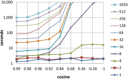
Fig. 7 displays execution times when LP-MERT constrains the outputwˆ to satisfycos(w0,wˆ) ≥ t, where t is on the x-axis of the figure. The figure shows that we can scale to 1000 sentences when (exactly) searching within the region defined by
[image:8.612.79.294.73.198.2]1 10 100 1,000 10,000
0.99 0.98 0.96 0.92 0.84 0.68 0.36 -0.28 -1
secon
d
s
1024 512 256
128 64 32 16 8 4
2 1
[image:9.612.75.295.74.212.2]cosine
Figure 7: Effect of a constraint onw(runtime on 1 CPU).
32 64 128 256 512 1024 1D-MERT 22.93 20.70 18.57 16.07 15.00 15.44 our work 25.25 22.28 19.86 17.05 15.56 15.67 +2.32 +1.59 +1.29 +0.98 +0.56 +0.23
Table 2: BLEUn4r1[%] scores for English-German on WMT09 for tuning sets ranging from 32 to 1024 sentences.
size. Results are displayed in Table 2. The gains are fairly substantial, with gains of 0.5 BLEU point or more in all cases whereS ≤ 512.8 Finally, we
perform an end-to-end MERT comparison, where both our algorithm and 1D-MERT are iteratively used to generate weights that in turn yield newN-best lists.
Tuning on 1024 sentences of WMT10, LP-MERT converges after seven iterations, with a BLEU score of 16.21%; 1D-MERT converges after nine iterations, with a BLEU score of 15.97%. Test set performance on the full WMT10 test set for LP-MERT and 1D-MERT are respectively 17.08% and 16.91%.
6 Related Work
One-dimensional MERT has been very influential. It is now used in a broad range of systems, and has been improved in a number of ways. For instance, lattices or hypergraphs may be used in place ofN-best lists to form a more comprehensive view of the search space with fewer decoding runs (Macherey et al., 2008; Kumar et al., 2009; Chatterjee and Cancedda, 2010). This particular refinement is orthogonal to our approach, though. We expect to extend LP-MERT
8One interesting observation is that the performance of
1D-MERT degrades asSgrows from 2 to 8 (Fig. 5), which contrasts with the results shown in Tab. 2. This may have to do with the fact thatN-best lists withS= 2have much fewer local maxima than withS = 4,8, in which case 20 restarts is generally enough.
to hypergraphs in future work. Exact search may be challenging due to the computational complexity of the search space (Leusch et al., 2008), but approxi-mate search should be feasible.
Other research has explored alternate methods of gradient-free optimization, such as the downhill-simplex algorithm (Nelder and Mead, 1965; Zens et al., 2007; Zhao and Chen, 2009). Although the search space is different than that of Och’s algorithm, it still relies on one-dimensional line searches to re-flect, expand, or contract the simplex. Therefore, it suffers the same problems of one-dimensional MERT: feature sets with complex non-linear interactions are difficult to optimize. LP-MERT improves on these methods by searching over a larger subspace of pa-rameter combinations, not just those on a single line. We can also change the objective function in a number of ways to make it more amenable to op-timization, leveraging knowledge from elsewhere in the machine learning community. Instance re-weighting as in boosting may lead to better param-eter inference (Duh and Kirchhoff, 2008). Smooth-ing the objective function may allow differentiation and standard ML learning techniques (Och and Ney, 2002). Smith and Eisner (2006) use a smoothed ob-jective along with deterministic annealing in hopes of finding good directions and climbing past locally optimal points. Other papers use margin methods such as MIRA (Watanabe et al., 2007; Chiang et al., 2008), updated somewhat to match the MT domain, to perform incremental training of potentially large numbers of features. However, in each of these cases the objective function used for training no longer matches the final evaluation metric.
7 Conclusions
Our primary contribution is the first known exact search algorithm for direct loss minimization onN
ap-plications. Recent speech recognition systems have also explored combinations of more acoustic and lan-guage models, with discriminative training of 5-10 features rather than one million (L¨o¨of et al., 2010); LP-MERT could be valuable here as well.
The one-dimensional algorithm of Och (2003) has been subject to study and refinement for nearly a decade, while this is the first study of multi-dimensional approaches. We demonstrate the poten-tial of multi-dimensional approaches, but we believe there is much room for improvement in both scalabil-ity and speed. Furthermore, a natural line of research would be to extend LP-MERT to compact representa-tions of the search space, such as hypergraphs.
There are a number of broader implications from this research. For instance, LP-MERT can aid in the evaluation of research on MERT. This approach sup-plies a truly optimal vector as ground truth, albeit under limited conditions such as a constrained direc-tion set, a reduced number of features, or a smaller set of sentences. Methods can be evaluated based on not only improvements over prior approaches, but also based on progress toward a global optimum.
Acknowledgements
We thank Xiaodong He, Kristina Toutanova, and three anonymous reviewers for their valuable sug-gestions.
Appendix A: Proof of optimality
In this appendix, we prove that LP-MERT (Algorithm 2) is exact. As noted before, the na¨ıve approach of solving Eq. 4 is to enumerate allO(NS)hypotheses combinations
inM, discard the ones that are not extreme, and return the best scoring one. LP-MERT relies on algorithmic improvements to speed up this approach, and we now show that none of them affect the optimality of the solution.
Divide-and-conquer. Divide-and-conquer in Algo-rithm 2 discards any partial hypothesis combination
h[m(j). . . m(k)]if it is not extreme, even before
consid-ering any extension h[m(i). . . m(j). . . m(k). . . m(l)].
This does not sacrifice optimality, since ifconv(h;H)
is false, thenconv(h;H∪G)is false for any setG.
Proof: Assumeconv(h;H)is false, sohis interior to
H. By definition, any interior pointhcan be written as
a linear combination of other points:h=Piλihi, with
∀i(hi∈H,hi6=h,λi ≥0)andPiλi= 1. This same
combination of points also demonstrates thathis interior
toH∪G, thusconv(h;H∪G)is false as well.
Sparse hypothesis combination. We show here that the simplification of linear programs in Section 3.1.1 from sizeO(NS)to size O(N S)does not change the
value ofconv(h;H). More specifically, this means that linear optimization of the output of the COMBINEmethod at lines 26-27 of function GETNEXTBEST does not introduce any error. Let (g1. . .gU) and (h1. . .hV) be
twoN-best lists to be combined, then:
conv
gu+hv; U
[
i=1
(gi+hv) ∪ V
[
j=1
(gu+hj)
=conv
gu+hv; U [ i=1 V [ j=1
(gi+hj)
Proof:To prove this equality, it suffices to show that: (1)
ifgu+hvis interior wrt. the firstconvbinary predicate
in the above equation, then it is interior wrt. the second conv, and (2) ifgu+hvis interior wrt. the secondconv,
then it is interior wrt. the firstconv. Claim (1) is evident, since the set of points in the firstconvis a subset of the other set of points. Thus, we only need to prove (2). We first geometrically translate all points by−gu−hv. Since
gu+hvis interior wrt. the secondconv, we can write:
0= U X i=1 V X j=1
λi,j(gi+hj−gu−hv)
= U X i=1 V X j=1
λi,j(gi−gu) + U X i=1 V X j=1
λi,j(hj−hv)
=
U
X
i=1
(gi−gu) V
X
j=1
λi,j+ V
X
j=1
(hj−hv) U X i=1 λi,j = U X i=1
λ0i(gi−gu) + V
X
j=1
λ0U+j(hj−hv)
where {λ0
i}1≤i≤U+V values are computed from
{λi,j}1≤i≤U,1≤j≤V as follows: λ0i =Pjλi,j, i∈[1, U]
and λ0
U+j =
P
iλi,j, j ∈ [1, V]. Since the interior
point is0,λ0ivalues can be scaled so that they sum to 1
(necessary condition in the definition of interior points), which proves that the following predicate is false:
conv 0; U [ i=1
(gi−gu) ∪ V
[
j=1
(hj−hv)
which is equivalent to stating that the following is false:
conv
gu+hv; U
[
i=1
(gi+hv) ∪ V
[
j=1
(gu+hj)
References
C. Bradford Barber, David P. Dobkin, and Hannu Huhdan-paa. 1996. The QuickHull algorithm for convex hulls.
ACM Trans. Math. Softw., 22:469–483.
C. Buchta, J. Muller, and R. F. Tichy. 1985. Stochastical approximation of convex bodies. Math. Ann., 271:225– 235.
A. Bykat. 1978. Convex hull of a finite set of points in two dimensions. Inf. Process. Lett., 7(6):296–298. Daniel Cer, Dan Jurafsky, and Christopher D. Manning.
2008. Regularization and search for minimum error rate training. InProceedings of the Third Workshop on Statistical Machine Translation, pages 26–34.
Samidh Chatterjee and Nicola Cancedda. 2010. Min-imum error rate training by sampling the translation lattice. InProceedings of the 2010 Conference on Em-pirical Methods in Natural Language Processing, pages 606–615. Association for Computational Linguistics. David Chiang, Yuval Marton, and Philip Resnik. 2008.
Online large-margin training of syntactic and structural translation features. InEMNLP.
David Chiang. 2007. Hierarchical phrase-based transla-tion. Computational Linguistics, 33(2):201–228. W. Chou, C. H. Lee, and B. H. Juang. 1993. Minimum
error rate training based on N-best string models. In
Proc. IEEE Int’l Conf. Acoustics, Speech, and Signal Processing (ICASSP ’93), pages 652–655, Vol. 2. Kevin Duh and Katrin Kirchhoff. 2008. Beyond
log-linear models: boosted minimum error rate training for programming N-best re-ranking. InProceedings of the 46th Annual Meeting of the Association for Computa-tional Linguistics on Human Language Technologies: Short Papers, pages 37–40, Stroudsburg, PA, USA. William F. Eddy. 1977. A new convex hull algorithm for
planar sets. ACM Trans. Math. Softw., 3:398–403. Liang Huang and David Chiang. 2005. Better k-best
pars-ing. InProceedings of the Ninth International Work-shop on Parsing Technology, pages 53–64, Stroudsburg, PA, USA.
Biing-Hwang Juang, Wu Hou, and Chin-Hui Lee. 1997. Minimum classification error rate methods for speech recognition. Speech and Audio Processing, IEEE Trans-actions on, 5(3):257–265.
N. Karmarkar. 1984. A new polynomial-time algorithm for linear programming. Combinatorica, 4:373–395. Victor Klee. 1966. Convex polytopes and linear
program-ming. InProceedings of the IBM Scientific Computing Symposium on Combinatorial Problems.
Philipp Koehn, Hieu Hoang, Alexandra Birch Mayne, Christopher Callison-Burch, Marcello Federico, Nicola Bertoldi, Brooke Cowan, Wade Shen, Christine Moran, Richard Zens, Chris Dyer, Ondrej Bojar, Alexandra Constantin, and Evan Herbst. 2007. Moses: Open
source toolkit for statistical machine translation. In
Proc. of ACL, Demonstration Session.
Shankar Kumar, Wolfgang Macherey, Chris Dyer, and Franz Och. 2009. Efficient minimum error rate train-ing and minimum Bayes-risk decodtrain-ing for translation hypergraphs and lattices. InProceedings of the Joint Conference of the 47th Annual Meeting of the ACL and the 4th International Joint Conference on Natural Language Processing of the AFNLP: Volume 1, pages 163–171.
Gregor Leusch, Evgeny Matusov, and Hermann Ney. 2008. Complexity of finding the BLEU-optimal hy-pothesis in a confusion network. InProceedings of the Conference on Empirical Methods in Natural Language Processing, pages 839–847, Stroudsburg, PA, USA. Zhifei Li, Chris Callison-Burch, Chris Dyer, Juri
Ganitke-vitch, Sanjeev Khudanpur, Lane Schwartz, Wren N. G. Thornton, Jonathan Weese, and Omar F. Zaidan. 2009. Joshua: an open source toolkit for parsing-based MT. InProc. of WMT.
P. Liang, A. Bouchard-Cˆot´e, D. Klein, and B. Taskar. 2006. An end-to-end discriminative approach to ma-chine translation. InInternational Conference on Com-putational Linguistics and Association for Computa-tional Linguistics (COLING/ACL).
Chin-Yew Lin and Franz Josef Och. 2004. ORANGE: a method for evaluating automatic evaluation metrics for machine translation. In Proceedings of the 20th international conference on Computational Linguistics, Stroudsburg, PA, USA.
Jonas L¨o¨of, Ralf Schl¨uter, and Hermann Ney. 2010. Dis-criminative adaptation for log-linear acoustic models. InINTERSPEECH, pages 1648–1651.
Wolfgang Macherey, Franz Och, Ignacio Thayer, and Jakob Uszkoreit. 2008. Lattice-based minimum error rate training for statistical machine translation. In Pro-ceedings of the 2008 Conference on Empirical Methods in Natural Language Processing, pages 725–734. David McAllester, Tamir Hazan, and Joseph Keshet. 2010.
Direct loss minimization for structured prediction. In
Advances in Neural Information Processing Systems 23, pages 1594–1602.
Ryan McDonald, Koby Crammer, and Fernando Pereira. 2005. Online large-margin training of dependency parsers. InProceedings of the 43rd Annual Meeting on Association for Computational Linguistics, pages 91–98.
Ryan McDonald. 2006. Discriminative sentence compres-sion with soft syntactic constraints. InProceedings of EACL, pages 297–304.
Conference on Computational Linguistics - Volume 1, pages 585–592.
J. A. Nelder and R. Mead. 1965. A simplex method for function minimization.Computer Journal, 7:308–313. Franz Josef Och and Hermann Ney. 2002. Discriminative
training and maximum entropy models for statistical machine translation. InProc. of the 40th Annual Meet-ing of the Association for Computational LMeet-inguistics, pages 295–302.
Franz Josef Och. 2003. Minimum error rate training for statistical machine translation. InProc. of ACL. Kishore Papineni, Salim Roukos, Todd Ward, and
Wei-Jing Zhu. 2001. BLEU: a method for automatic evalu-ation of machine translevalu-ation. InProc. of ACL.
M.J.D. Powell. 1964. An efficient method for finding the minimum of a function of several variables without calculating derivatives. Comput. J., 7(2):155–162. William H. Press, Saul A. Teukolsky, William T.
Vetter-ling, and Brian P. Flannery. 2007. Numerical Recipes: The Art of Scientific Computing. Cambridge University Press, 3rd edition.
Chris Quirk, Arul Menezes, and Colin Cherry. 2005. Dependency treelet translation: syntactically informed phrasal SMT. InProc. of ACL, pages 271–279. David A. Smith and Jason Eisner. 2006. Minimum risk
annealing for training log-linear models. In Proceed-ings of the COLING/ACL on Main conference poster sessions, pages 787–794, Stroudsburg, PA, USA. Matthew Snover, Bonnie Dorr, Richard Schwartz,
Lin-nea Micciulla, and John Makhoul. 2006. A study of translation edit rate with targeted human annotation. In
Proc. of AMTA, pages 223–231.
Andreas Stolcke, Yochai Knig, and Mitchel Weintraub. 1997. Explicit word error minimization in N-best list rescoring. InIn Proc. Eurospeech, pages 163–166. Taro Watanabe, Jun Suzuki, Hajime Tsukada, and Hideki
Isozaki. 2007. Online large-margin training for statisti-cal machine translation. InEMNLP-CoNLL.
Omar F. Zaidan and Chris Callison-Burch. 2009. Feasibil-ity of human-in-the-loop minimum error rate training. InProceedings of the 2009 Conference on Empirical Methods in Natural Language Processing: Volume 1 -Volume 1, pages 52–61.
Richard Zens, Sasa Hasan, and Hermann Ney. 2007. A systematic comparison of training criteria for sta-tistical machine translation. In Proceedings of the 2007 Joint Conference on Empirical Methods in Natu-ral Language Processing and Computational NatuNatu-ral Language Learning (EMNLP-CoNLL), pages 524–532, Prague, Czech Republic.
Bing Zhao and Shengyuan Chen. 2009. A simplex Armijo downhill algorithm for optimizing statistical machine translation decoding parameters. InProceedings of