Feature Noising for Log Linear Structured Prediction

Feature Noising for Log-linear Structured Prediction

Sida I. Wang∗, Mengqiu Wang∗, Stefan Wager†, Percy Liang, Christopher D. Manning

Department of Computer Science, †Department of Statistics Stanford University, Stanford, CA 94305, USA

{sidaw, mengqiu, pliang, manning}@cs.stanford.edu [email protected]

Abstract

NLP models have many and sparse features, and regularization is key for balancing model overfitting versus underfitting. A recently re-popularized form of regularization is to gen-erate fake training data by repeatedly adding noise to real data. We reinterpret this noising as an explicit regularizer, and approximate it with a second-order formula that can be used during training without actually generating fake data. We show how to apply this method to structured prediction using multinomial lo-gistic regression and linear-chain CRFs. We tackle the key challenge of developing a dy-namic program to compute the gradient of the regularizer efficiently. The regularizer is a sum over inputs, so we can estimate it more accurately via a semi-supervised or transduc-tive extension. Applied to text classification and NER, our method provides a>1% abso-lute performance gain over use of standardL2 regularization.

1 Introduction

NLP models often have millions of mainly sparsely attested features. As a result, balancing overfitting versus underfitting through good weight regulariza-tion remains a key issue for achieving optimal per-formance. Traditionally, L2 orL1 regularization is

employed, but these simple types of regularization penalize all features in a uniform way without tak-ing into account the properties of the actual model.

An alternative approach to regularization is to generate fake training data by adding random noise to the input features of the original training data. In-tuitively, this can be thought of as simulating

miss-∗

Both authors contributed equally to the paper

ing features, whether due to typos or use of a pre-viously unseen synonym. The effectiveness of this technique is well-known in machine learning (Abu-Mostafa, 1990; Burges and Sch¨olkopf, 1997; Simard et al., 2000; Rifai et al., 2011a; van der Maaten et al., 2013), but working directly with many cor-rupted copies of a dataset can be computationally prohibitive. Fortunately, feature noising ideas often lead to tractable deterministic objectives that can be optimized directly. Sometimes, training with cor-rupted features reduces to a special form of reg-ularization (Matsuoka, 1992; Bishop, 1995; Rifai et al., 2011b; Wager et al., 2013). For example, Bishop (1995) showed that training with features that have been corrupted with additive Gaussian noise is equivalent to a form ofL2regularization in

the low noise limit. In other cases it is possible to develop a new objective function by marginalizing over the artificial noise (Wang and Manning, 2013; van der Maaten et al., 2013).

The central contribution of this paper is to show how to efficiently simulate training with artificially noised features in the context of log-linear struc-tured prediction, without actually having to gener-ate noised data. We focus on dropout noise (Hinton et al., 2012), a recently popularized form of artifi-cial feature noise where a random subset of features is omitted independently for each training example. Dropout and its variants have been shown to out-performL2 regularization on various tasks (Hinton

et al., 2012; Wang and Manning, 2013; Wan et al., 2013). Dropout is is similar in spirit to feature bag-ging in the deliberate removal of features, but per-forms the removal in a preset way rather than ran-domly (Bryll et al., 2003; Sutton et al., 2005; Smith et al., 2005).

Our approach is based on a second-order approx-imation to feature noising developed among others by Bishop (1995) and Wager et al. (2013), which al-lows us to convert dropout noise into a form of adap-tive regularization. This method is suitable for struc-tured prediction in log-linear models where second derivatives are computable. In particular, it can be used for multiclass classification with maximum en-tropy models (a.k.a., softmax or multinomial logis-tic regression) and for the sequence models that are ubiquitous in NLP, via linear chain Conditional Ran-dom Fields (CRFs).

For linear chain CRFs, we additionally show how we can use a noising scheme that takes advantage of the clique structure so that the resulting noising regularizer can be computed in terms of the pair-wise marginals. A simple forward-backward-type dynamic program can then be used to compute the gradient tractably. For ease of implementation and scalability to semi-supervised learning, we also out-line an even faster approximation to the regularizer. The general approach also works in other clique structures in addition to the linear chain when the clique marginals can be computed efficiently.

Finally, we extend feature noising for structured prediction to a transductive or semi-supervised set-ting. The regularizer induced by feature noising is label-independent for log-linear models, and so we can use unlabeled data to learn a better regu-larizer. NLP sequence labeling tasks are especially well suited to a semi-supervised approach, as input features are numerous but sparse, and labeled data is expensive to obtain but unlabeled data is abundant (Li and McCallum, 2005; Jiao et al., 2006).

Wager et al. (2013) showed that semi-supervised dropout training for logistic regression captures a similar intuition to techniques such as entropy regu-larization (Grandvalet and Bengio, 2005) and trans-ductive SVMs (Joachims, 1999), which encourage confident predictions on the unlabeled data. Semi-supervised dropout has the advantage of only us-ing the predicted label probabilities on the unlabeled data to modulate an L2 regularizer, rather than

re-quiring more heavy-handed modeling of the unla-beled data as in entropy regularization or expecta-tion regularizaexpecta-tion (Mann and McCallum, 2007).

In experimental results, we show that simulated feature noising gives more than a 1% absolute boost

y

y

y

f

(

y

,

x

)

f

(

y

,

y

)

f

(

y

,

y

)

y

y

y

f

(y

,

x

)

f

(

y

,

y

)

f

(

y

,

y

)

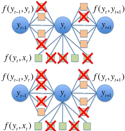
Figure 1: An illustration of dropout feature noising in linear-chain CRFs with only transition features and node features. The green squares are node fea-turesf(yt, xt), and the orange squares are edge

fea-turesf(yt−1, yt). Conceptually, given a training

ex-ample, we sample some features to ignore (generate fake data) and make a parameter update. Our goal is to train with a roughly equivalent objective, without actually sampling.

in performance overL2 regularization, on both text

classification and an NER sequence labeling task.

2 Feature Noising Log-linear Models

Consider the standard structured prediction problem of mapping some input x ∈ X (e.g., a sentence) to an output y ∈ Y (e.g., a tag sequence). Let

f(y, x) ∈ _Rd_{be the feature vector, θ ∈}

Rdbe the weight vector, ands= (s1, . . . , s|Y|)be a vector of

scores for each output, withsy =f(y, x)·θ. Now

define a log-linear model:

p(y|x;θ) = exp{sy−A(s)}, (1)

whereA(s) = logP

yexp{sy}is the log-partition

function. Given an example(x,y), parameter esti-mation corresponds to choosingθto maximizep(y|

x;θ).

into some f˜(y, x) and then maximize the average log-likelihood ofygiven these corrupted features— the motivation is to choose predictorsθthat are ro-bust to noise (missing words for example). Let˜s, ˜

p(y|x;θ)be therandomlyperturbed versions cor-responding to f˜(y, x). We will also assume the feature noising preserves the mean: E[ ˜f(y, x)] =

f(y, x), so thatE[˜s] = s. This can always be done by scaling the noised features as described in the list of noising schemes.

It is useful to view feature noising as a form of regularization. Since feature noising preserves the mean, the feature noising objective can be written as the sum of the original log-likelihood plus the dif-ference in log-normalization constants:

E[log ˜p(y|x;θ)] =E[˜sy−A(˜s)] (2)

= logp(y|x;θ)−R(θ, x), (3)

R(θ, x)def= E[A(˜s)]−A(s). (4)

SinceA(·) is convex,R(θ, x)is always positive by Jensen’s inequality and can therefore be interpreted as a regularizer. Note thatR(θ, x)is in general non-convex.

Computing the regularizer (4) requires summing over all possible noised feature vectors, which can imply exponential effort in the number of features. This is intractable even for flat classification. Fol-lowing Bishop (1995) and Wager et al. (2013), we approximate R(θ, x) using a second-order Taylor expansion, which will allow us to work with only means and covariances of the noised features. We take a quadratic approximation of the log-partition function A(·) of the noised score vector ˜s around the the unnoised score vectors:

A(˜s)uA(s) +∇A(s)>(˜s−s) (5)

+1

2(˜s−s)

>_∇2_{A(s)(˜s−s).}

Plugging (5) into (4), we obtain a new regularizer

Rq(θ, x), which we will use as an approximation to

R(θ, x):

Rq(θ, x) = 1

2E[(˜s−s)

>_∇2_{A(s)(˜s−s)] (6)}

= 1

2tr(∇

2_{A(s) Cov(˜s)). (7)}

This expression still has two sources of potential in-tractability, a sum over an exponential number of noised score vectors˜sand a sum over the|Y| com-ponents of˜s.

Multiclass classification If we assume that the components of ˜s are independent, then Cov(˜s) ∈ R|Y|×|Y|is diagonal, and we have

Rq(θ, x) = 1 2

X

y∈Y

µy(1−µy) Var[˜sy], (8)

where the meanµy

def

= pθ(y |x)is the model

prob-ability, the varianceµy(1−µy)measures model

un-certainty, and

Var[˜sy] =θ>Cov[ ˜f(y, x)]θ (9)

measures the uncertainty caused by feature noising.1 The regularizerRq(θ, x)involves the product of two variance terms, the first is non-convex inθand the second is quadratic inθ. Note that to reduce the reg-ularization, we will favor models that (i) predict con-fidently and (ii) have stable scores in the presence of feature noise.

For multiclass classification, we can explicitly sum over each y ∈ Y to compute the regularizer, but this will be intractable for structured prediction. To specialize to multiclass classification for the moment, let us assume that we have a separate weight vector for each outputyapplied to the same feature vectorg(x); that is, the scoresy=θy·g(x).

Further, assume that the components of the noised feature vectorg˜(x) are independent. Then we can simplify (9) to the following:

Var[˜sy] =

X

j

Var[gj(x)]θ2yj. (10)

Noising schemes We now give some examples of possible noise schemes for generatingf˜(y, x)given the original features f(y, x). This distribution af-fects the regularization through the variance term Var[˜sy].

• Additive Gaussian: ˜

f(y, x) = f(y, x) + ε, where ε ∼ N(0, σ2Id×d).

1

In this case, the contribution to the regularizer from noising isVar[˜sy] =P_jσ2θ2_yj.

• Dropout:

˜

f(y, x) = f(y, x)z, wheretakes the el-ementwise product of two vectors. Here,z is a vector with independent components which haszi = 0with probability δ, zi = ₁₋1_δ with

probability 1 − δ. In this case, Var[˜sy] =

P

j gj(x)2δ

1−δ θ

2

yj.

• Multiplicative Gaussian:

˜

f(y, x) = f(y, x) (1 + ε), where

ε ∼ N(0, σ2_I

d×d). Here, Var[˜sy] =

P

jgj(x)2σ2θ2yj. Note that under our

second-order approximation Rq(θ, x), the multiplica-tive Gaussian and dropout schemes are equiva-lent, but they differ under the original regular-izerR(θ, x).

2.1 Semi-supervised learning

A key observation (Wager et al., 2013) is that the noising regularizer R (8), while involving a sum over examples, is independent of the output

y. This suggests estimating R using unlabeled data. Specifically, if we have n labeled examples

D = {x1, x2, . . . , xn} and m unlabeled examples D_unlabeled ={u1, u2, . . . , un}, then we can define a

regularizer that is a linear combination the regular-izer estimated on both datasets, with α tuning the tradeoff between the two:

R∗(θ,D,D_unlabeled) (11)

def

= n

n+αm

Xn

i=1

R(θ, xi) +α m

X

i=1

R(θ, ui)

.

3 Feature Noising in Linear-Chain CRFs

So far, we have developed a regularizer that works for all log-linear models, but—in its current form— is only practical for multiclass classification. We now exploit the decomposable structure in CRFs to define a new noising scheme which does not require us to explicitly sum over all possible outputsy∈ Y. The key idea will be to noise each local feature vec-tor (which implicitly affects many y) rather than noise eachyindependently.

Assume that the outputy= (y1, . . . , yT)is a

se-quence ofT tags. In linear chain CRFs, the feature vectorfdecomposes into a sum of local feature vec-torsgt:

f(y, x) =

T

X

t=1

gt(yt−1, yt, x), (12)

wheregt(a, b, x)is defined on a pair of consecutive

tagsa, bfor positionst−1andt.

Rather than working with a score sy for each

y ∈ Y, we define a collection of local scores

s = {sa,b,t}, for each tag pair (a, b) and

posi-tion t = 1, . . . , T. We consider noising schemes which independently set g˜t(a, b, x) for each a, b, t.

Let˜s = {s˜a,b,t}be the corresponding collection of

noised scores.

We can write the log-partition function of these local scores as follows:

A(s) = logX

y∈Y

exp ( _T

X

t=1

syt−1,yt,t )

. (13)

The first derivative yields the edge marginals under the model,µa,b,t = pθ(yt−1 = a, yt = b | x), and

the diagonal elements of the Hessian∇2_A(s)yield

the marginal variances.

Now, following (7) and (8), we obtain the follow-ing regularizer:

Rq(θ, x) = 1 2

X

a,b,t

µa,b,t(1−µa,b,t) Var[˜sa,b,t],

(14)

whereµa,b,t(1−µa,b,t)measures model uncertainty

about edge marginals, andVar[˜sa,b,t]is simply the

uncertainty due to noising. Again, minimizing the regularizer means making confident predictions and having stable scores under feature noise.

Computing partial derivatives So far, we have defined the regularizer Rq(θ, x) based on feature noising. In order to minimizeRq(θ, x), we need to take its derivative.

First, note thatlogµa,b,tis the difference of a

re-stricted log-partition function and the log-partition function. So again by properties of its first deriva-tive, we have:

∇logµa,b,t=Epθ(y|x,yt−1=a,yt=b)[f(y, x)] (15)

Using the fact that ∇µa,b,t = µa,b,t∇logµa,b,t and

the fact thatVar[˜sa,b,t]is a quadratic function inθ,

we can simply apply the product rule to derive the final gradient∇Rq(θ, x).

3.1 A Dynamic Program for the Conditional Expectation

A naive computation of the gradient∇Rq_{(θ, x)} re-quires a full forward-backward pass to compute Epθ(y|yt−1=a,yt=b,x)[f(y, x)]for each tag pair(a, b) and position t, resulting in a O(K4T2) time algo-rithm.

In this section, we reduce the running time to

O(K2T) using a more intricate dynamic program. By the Markov property of the CRF,y1:t−2only

de-pends on (yt−1, yt) through yt−1 and yt+1:T only

depends on(yt−1, yt)throughyt.

First, it will be convenient to define the partial sum of the local feature vector from positions ito

jas follows:

Gi:j = j

X

t=i

gt(yt−1, yt, x). (16)

Consider the task of computing the feature expecta-tion Epθ(y|yt−1=a,yt=b)[f(y, x)]for a fixed (a, b, t). We can expand this quantity into

X

y:yt−1=a,yt=b

pθ(y−(t−1:t) |yt−1 =a, yt=b)G1:T.

Conditioning onyt−1, yt decomposes the sum into

three pieces:

X

y:yt−1=a,yt=b

[gt(yt−1 =a, yt=b, x) +Fta+Btb],

where

F_ta= X

y1:t−2

pθ(y1:t−2|yt−1=a)G1:t−1, (17)

Bb_t = X

yt+1:T

pθ(yt+1:T |yt=b)Gt+1:T, (18)

are the expected feature vectors summed over the prefix and suffix of the tag sequence, respectively. Note thatF_ta andB_tb are analogous to the forward and backward messages of standard CRF inference, with the exception that they are vectors rather than scalars.

We can compute these messages recursively in the standard way. The forward recurrence is

F_ta=X

b

pθ(yt−2 =b|yt−1 =a)

h

gt(yt−2 =b, yt−1 =a, x) +Ftb−1

i

,

and a similar recurrence holds for the backward mes-sagesB_tb.

Running the resulting dynamic program takes

O(K2T q) time and requires O(KT q) storage, whereK is the number of tags, T is the sequence length andq is the number of active features. Note that this is the same order of dependence as normal CRF training, but there is an additional dependence on the number of active features q, which makes training slower.

4 Fast Gradient Computations

In this section, we provide two ways to further im-prove the efficiency of the gradient calculation based on ignoring long-range interactions and based on ex-ploiting feature sparsity.

4.1 Exploiting Feature Sparsity and Co-occurrence

In each forward-backward pass over a training ample, we need to compute the conditional ex-pectations for all features active in that example. Naively applying the dynamic program in Section 3 isO(K2T)for each active feature. The total com-plexity has to factor in the number of active fea-tures, q. Although q only scales linearly with sen-tence length, in practice this number could get large pretty quickly. For example, in the NER tagging ex-periments (cf. Section 5), the average number of active features per token is about 20, which means

q ' 20T; this term quickly dominates the compu-tational costs. Fortunately, in sequence tagging and other NLP tasks, the majority of features are sparse and they often co-occur. That is, some of the ac-tive features would fire and only fire at the same lo-cations in a given sequence. This happens when a particular token triggers multiple rare features.

feature as a preprocessing step to avoid computing identical expectations for each of the features. Do-ing so on the same NER taggDo-ing experiments cuts downq/T from 20 to less than 5, and gives us a 4 times speed up at no loss of accuracy. The exact same trick is applicable to the general CRF gradient computation as well and gives similar speedup.

4.2 Short-range interactions

It is also possible to speed up the method by re-sorting to approximate gradients. In our case, the dynamic program from Section 3 together with the trick described above ran in a manageable amount of time. The techniques developed here, however, could prove to be useful on larger tasks.

Let us rewrite the quantity we want to compute slightly differently (again, for alla, b, t):

T

X

i=1

Epθ(y|x,yt−1=a,yt=b)[gi(yi−1, yi, x)]. (19)

The intuition is that conditioned on yt−1, yt, the

terms gi(yi−1, yi, x) where i is far from t will be

close toEpθ(y|x)[gi(yi−1, yi, x)].

This motivates replacing the former with the latter whenever|i−k| ≥rwhereris some window size. This approximation results in an expression which only has to consider the sum of the local feature vec-tors fromi−rtoi+r, which is captured byGi−r:i+r:

Epθ(y|yt−1=a,yt=b,x)[f(y, x)]−Epθ(y|x)[f(y, x)] ≈_Ep

θ(y|yt−1=a,yt=b,x)[Gt−r:t+r] (20) −Epθ(y|x)[Gt−r:t+r].

We can further approximate this last expression by lettingr= 0, obtaining:

gt(a, b, x)−Epθ(y|x)[gt(yt−1, yt, x)]. (21)

The second expectation can be computed from the edge marginals.

The accuracy of this approximation hinges on the lack of long range dependencies. Equation (21) shows the case ofr = 0; this takes almost no addi-tional effort to compute. However, for some of our experiments, we observed a 20% difference with the real derivative. Forr >0, the computational savings are more limited, but the bounded-window method is easier to implement.

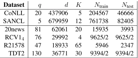
Dataset q d K Ntrain Ntest CoNLL 20 437906 5 204567 46666 SANCL 5 679959 12 761738 82405 20news 81 62061 20 15935 3993 RCV14 76 29992 4 9625/2 9625/2

R21578 47 18933 65 5946 2347 TDT2 130 36771 30 9394/2 9394/2

Table 1: Description of datasets.q: average number of non-zero features per example, d: total number of features,K: number of classes to predict,Ntrain: number of training examples,Ntest: number of test examples.

5 Experiments

We show experimental results on the CoNLL-2003 Named Entity Recognition (NER) task, the SANCL Part-of-speech (POS) tagging task, and several doc-ument classification tasks.2 The datasets used are described in Table 1. We used standard splits when-ever available; otherwise we split the data at ran-dom into a test set and a train set of equal sizes (RCV14, TDT2). CoNLL has a development set

of size 51578, which we used to tune regulariza-tion parameters. The SANCL test set is divided into 3 genres, namely answers, newsgroups, and

reviews, each of which has a corresponding de-velopment set.3

5.1 Multiclass Classification

We begin by testing our regularizer in the simple case of classification whereY ={1,2, . . . , K}for

Kclasses. We examine the performance of the nois-ing regularizer in both the fully supervised settnois-ing as well as the transductive learning setting.

In the transductive learning setting, the learner is allowed to inspect the test features at train time (without the labels). We used the method described in Section 2.1 for transductive dropout.

Dataset K None L2 Drop +Test

CoNLL 5 78.03 80.12 80.90 81.66 20news 20 81.44 82.19 83.37 84.71 RCV14 4 95.76 95.90 96.03 96.11

R21578 65 92.24 92.24 92.24 92.58 TDT2 30 97.74 97.91 98.00 98.12

Table 2: Classification performance and transduc-tive learning results on some standard datasets. None: use no regularization, Drop: quadratic ap-proximation to the dropout noise (8), +Test: also use the test set to estimate the noising regularizer (11).

5.1.1 Semi-supervised Learning with Feature Noising

In the transductive setting, we used test data (without labels) to learn a better regularizer. As an alternative, we could also use unlabeled data in place of the test data to accomplish a similar goal; this leads to a semi-supervised setting.

To test the semi-supervised idea, we use the same datasets as above. We split each dataset evenly into 3 thirds that we use as a training set, a test set and an unlabeled dataset. Results are given in Table 3.

In most cases, our semi-supervised accuracies are lower than the transductive accuracies given in Table 2; this is normal in our setup, because we used less labeled data to train the semi-supervised classifier than the transductive one.4

5.1.2 The Second-Order Approximation

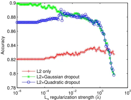
The results reported above all rely on the ap-proximate dropout regularizer (8) that is based on a second-order Taylor expansion. To test the validity of this approximation we compare it to the Gaussian method developed by Wang and Manning (2013) on a two-class classification task.

We use the 20-newsgroups alt.atheism vs

soc.religion.christianclassification task; results are shown in Figure 2. There are 1427

exam-4_{The CoNNL results look somewhat surprising, as the} semi-supervised results are better than the transductive ones. The reason for this is that the original CoNLL test set came from a different distributions than the training set, and this made the task more difficult. Meanwhile, in our semi-supervised experi-ment, the test and train sets are drawn from the same distribu-tion and so our semi-supervised task is actually easier than the original one.

Dataset K L2 Drop +Unlabeled

CoNLL 5 91.46 91.81 92.02 20news 20 76.55 79.07 80.47 RCV14 4 94.76 94.79 95.16

R21578 65 90.67 91.24 90.30 TDT2 30 97.34 97.54 97.89

Table 3: Semisupervised learning results on some standard datasets. A third (33%) of the full dataset was used for training, a third for testing, and the rest as unlabeled.

10−6 10−4 10−2 100 102

0.78 0.8 0.82 0.84 0.86 0.88 0.9

L

2 regularization strength (λ)

Accuracy

L2 only

L2+Gaussian dropout L2+Quadratic dropout

Figure 2: Effect ofλinλkθk2

2on the testset

perfor-mance. Plotted is the test set accuracy with logis-tic regression as a function ofλfor theL2

regular-izer, Gaussian dropout (Wang and Manning, 2013) + additionalL2, and quadratic dropout (8) +L2

de-scribed in this paper. The default noising regularizer is quite good, and additionalL2does not help.

No-tice that no choice ofλ inL2 can help us combat

overfitting as effectively as (8) without underfitting.

ples with 22178 features, split evenly and randomly into a training set and a test set.

Over a broad range of λ values, we find that dropout plus L2 regularization performs far better

computational efficiency and prediction accuracy.

5.2 CRF Experiments

We evaluate the quadratic dropout regularizer in linear-chain CRFs on two sequence tagging tasks: the CoNLL 2003 NER shared task (Tjong Kim Sang and De Meulder, 2003) and the SANCL 2012 POS tagging task (Petrov and McDonald, 2012) .

The standard CoNLL-2003 English shared task benchmark dataset (Tjong Kim Sang and De Meul-der, 2003) is a collection of documents from Reuters newswire articles, annotated with four en-tity types: Person, Location, Organization, and Miscellaneous. We predicted the label sequence

Y = {LOC, MISC, ORG, PER, O}T _without

con-sidering the BIO tags.

For training the CRF model, we used a compre-hensive set of features from Finkel et al. (2005) that gives state-of-the-art results on this task. A total number of 437906 features were generated on the CoNLL-2003 training dataset. The most important features are:

• The word, word shape, and letter n-grams (up to 6gram) at current position

• The prediction, word, and word shape of the pre-vious and next position

• Previous word shape in conjunction with current word shape

• Disjunctive word set of the previous and next 4 positions

• Capitalization pattern in a 3 word window

• Previous two words in conjunction with the word shape of the previous word

• The current word matched against a list of name titles (e.g., Mr., Mrs.)

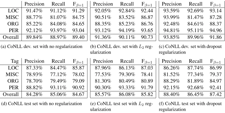
The Fβ=1 results are summarized in Table 4. We

obtain a 1.6% and 1.1% absolute gain on the test and dev set, respectively. Detailed results are bro-ken down by precision and recall for each tag and are shown in Table 6. These improvements are signifi-cant at the 0.1% level according to the paired boot-strap resampling method of 2000 iterations (Efron and Tibshirani, 1993).

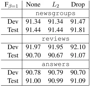
For the SANCL (Petrov and McDonald, 2012) POS tagging task, we used the same CRF framework with a much simpler set of features

• word unigrams: w−1, w0, w1

• word bigram: (w−1, w0) and (w0, w1)

Fβ=1 None L2 Drop

Dev 89.40 90.73 91.86 Test 84.67 85.82 87.42

Table 4: CoNLL summary of results. None: no reg-ularization, Drop: quadratic dropout regularization (14) described in this paper.

Fβ=1 None L2 Drop

newsgroups

Dev 91.34 91.34 91.47 Test 91.44 91.44 91.81

reviews

Dev 91.97 91.95 92.10 Test 90.70 90.67 91.07

answers

Dev 90.78 90.79 90.70 Test 91.00 90.99 91.09

Table 5: SANCL POS taggingFβ=1scores for the 3

official evaluation sets.

We obtained a small but consistent improvement using the quadratic dropout regularizer in (14) over theL2-regularized CRFs baseline.

Although the difference on SANCL is small, the performance differences on the test sets of

reviews andnewsgroups are statistically sig-nificant at the 0.1% level. This is also interesting because here is a situation where the features are ex-tremely sparse,L2 regularization gave no

improve-ment, and where regularization overall matters less.

6 Conclusion

Inves-Precision Recall Fβ=1

LOC 91.47% 91.12% 91.29 MISC 88.77% 81.07% 84.75 ORG 85.22% 84.08% 84.65 PER 92.12% 93.97% 93.04 Overall 89.84% 88.97% 89.40

(a) CoNLL dev. set with no regularization

Precision Recall Fβ=1

92.05% 92.84% 92.44 90.51% 83.52% 86.87 88.35% 85.23% 86.76 93.12% 94.19% 93.65 91.36% 90.11% 90.73

(b) CoNLL dev. set withL2 reg-ularization

Precision Recall Fβ=1

93.59% 92.69% 93.14 93.99% 81.47% 87.28 92.48% 84.61% 88.37 94.81% 95.11% 94.96 93.85% 89.96% 91.86

(c) CoNLL dev. set with dropout regularization

Tag Precision Recall Fβ=1

LOC 87.33% 84.47% 85.87 MISC 78.93% 77.12% 78.02 ORG 78.70% 79.49% 79.09 PER 88.82% 93.11% 90.92 Overall 84.28% 85.06% 84.67

(d) CoNLL test set with no regularization

Precision Recall Fβ=1

87.96% 86.13% 87.03 77.53% 79.30% 78.41 81.30% 80.49% 80.89 90.30% 93.33% 91.79 85.57% 86.08% 85.82

(e) CoNLL test set withL2 reg-ularization

Precision Recall Fβ=1

86.26% 87.74% 86.99 81.52% 77.34% 79.37 88.29% 81.89% 84.97 92.15% 92.68% 92.41 88.40% 86.45% 87.42

(f) CoNLL test set with dropout regularization

Table 6: CoNLL NER results broken down by tags and by precision, recall, and Fβ=1. Top: development

set, bottom: test set performance.

tigating how to better optimize this non-convex reg-ularizer online and convincingly scale it to the semi-supervised setting seem to be promising future di-rections.

Acknowledgements

The authors would like to thank the anonymous re-viewers for their comments. We gratefully acknowl-edge the support of the Defense Advanced Research Projects Agency (DARPA) Broad Operational Lan-guage Translation (BOLT) program through IBM. Any opinions, findings, and conclusions or recom-mendations expressed in this material are those of the author(s) and do not necessarily reflect the view of the DARPA, or the US government. S. Wager is supported by a BC and EJ Eaves SGF Fellowship.

References

Yaser S. Abu-Mostafa. 1990. Learning from hints in neural networks. Journal of Complexity, 6(2):192– 198.

Chris M. Bishop. 1995. Training with noise is equiva-lent to Tikhonov regularization. Neural computation, 7(1):108–116.

Robert Bryll, Ricardo Gutierrez-Osuna, and Francis Quek. 2003. Attribute bagging: improving accuracy

of classifier ensembles by using random feature sub-sets. Pattern recognition, 36(6):1291–1302.

Chris J.C. Burges and Bernhard Sch¨olkopf. 1997. Im-proving the accuracy and speed of support vector ma-chines. InAdvances in Neural Information Processing Systems, pages 375–381.

Brad Efron and Robert Tibshirani. 1993.An Introduction to the Bootstrap. Chapman & Hall, New York. Jenny Rose Finkel, Trond Grenager, and Christopher

Manning. 2005. Incorporating non-local informa-tion into informainforma-tion extracinforma-tion systems by Gibbs sam-pling. In Proceedings of the 43rd annual meeting of the Association for Computational Linguistics, pages 363–370.

Yves Grandvalet and Yoshua Bengio. 2005. Entropy regularization. InSemi-Supervised Learning, United Kingdom. Springer.

Geoffrey E. Hinton, Nitish Srivastava, Alex Krizhevsky, Ilya Sutskever, and Ruslan R. Salakhutdinov. 2012. Improving neural networks by preventing co-adaptation of feature detectors. arXiv preprint arXiv:1207.0580.

text classification using support vector machines. In Proceedings of the International Conference on Ma-chine Learning, pages 200–209.

Wei Li and Andrew McCallum. 2005. Semi-supervised sequence modeling with syntactic topic models. In Proceedings of the 20th national conference on Arti-ficial Intelligence - Volume 2, AAAI’05, pages 813– 818.

Gideon S. Mann and Andrew McCallum. 2007. Sim-ple, robust, scalable semi-supervised learning via ex-pectation regularization. InProceedings of the Inter-national Conference on Machine Learning.

Kiyotoshi Matsuoka. 1992. Noise injection into inputs in back-propagation learning. Systems, Man and Cy-bernetics, IEEE Transactions on, 22(3):436–440.

Slav Petrov and Ryan McDonald. 2012. Overview of the 2012 shared task on parsing the web. Notes of the First Workshop on Syntactic Analysis of Non-Canonical Language (SANCL).

Salah Rifai, Yann Dauphin, Pascal Vincent, Yoshua Ben-gio, and Xavier Muller. 2011a. The manifold tangent classifier. Advances in Neural Information Processing Systems, 24:2294–2302.

Salah Rifai, Xavier Glorot, Yoshua Bengio, and Pascal Vincent. 2011b. Adding noise to the input of a model trained with a regularized objective. arXiv preprint arXiv:1104.3250.

Patrice Y. Simard, Yann A. Le Cun, John S. Denker, and Bernard Victorri. 2000. Transformation invariance in pattern recognition: Tangent distance and propagation. International Journal of Imaging Systems and Tech-nology, 11(3):181–197.

Andrew Smith, Trevor Cohn, and Miles Osborne. 2005. Logarithmic opinion pools for conditional random fields. InProceedings of the 43rd Annual Meeting on Association for Computational Linguistics, pages 18– 25. Association for Computational Linguistics.

Charles Sutton, Michael Sindelar, and Andrew McCal-lum. 2005. Feature bagging: Preventing weight un-dertraining in structured discriminative learning. Cen-ter for Intelligent Information Retrieval, U. of Mas-sachusetts.

Erik F. Tjong Kim Sang and Fien De Meulder. 2003. Introduction to the conll-2003 shared task: language-independent named entity recognition. InProceedings of the seventh conference on Natural language learn-ing at HLT-NAACL 2003 - Volume 4, CONLL ’03, pages 142–147.

Laurens van der Maaten, Minmin Chen, Stephen Tyree, and Kilian Q. Weinberger. 2013. Learning with marginalized corrupted features. InProceedings of the International Conference on Machine Learning.

Stefan Wager, Sida Wang, and Percy Liang. 2013. Dropout training as adaptive regularization. arXiv preprint:1307.1493.

Li Wan, Matthew Zeiler, Sixin Zhang, Yann LeCun, and Rob Fergus. 2013. Regularization of neural networks using dropconnect. In Proceedings of the Interna-tional Conference on Machine learning.