Weakly-Supervised Learning with
Cost-Augmented Contrastive Estimation
Kevin Gimpel Mohit Bansal
Toyota Technological Institute at Chicago, IL 60637, USA
{kgimpel,mbansal}@ttic.edu
Abstract
We generalize contrastive estimation in two ways that permit adding more knowl-edge to unsupervised learning. The first allows the modeler to specify not only the
set of corrupted inputs for each observa-tion, but also how bad each one is. The second allows specifying structural prefer-ences on the latent variable used to explain the observations. They require setting ad-ditional hyperparameters, which can be problematic in unsupervised learning, so we investigate new methods for unsuper-vised model selection and system com-bination. We instantiate these ideas for part-of-speech induction without tag dic-tionaries, improving over contrastive esti-mation as well as strong benchmarks from the PASCAL 2012 shared task.
1 Introduction
Unsupervised NLP aims to discover useful struc-ture in unannotated text. This strucstruc-ture might be part-of-speech (POS) tag sequences (Merialdo, 1994), morphological segmentation (Creutz and Lagus, 2005), or syntactic structure (Klein and Manning, 2004), among others. Unsupervised systems typically improve when researchers incor-porate knowledge to bias learning to capture char-acteristics of the desired structure.1
There are many successful examples of adding knowledge to improve learning without labeled examples, including: sparsity in POS tag distri-butions (Johnson, 2007; Ravi and Knight, 2009; Ganchev et al., 2010), short attachments for dependency parsing (Smith and Eisner, 2006),
1We note that doing so strains the definition of the term
unsupervised. Hence we will use the termweakly-supervised to refer to methods that do not explicitly train on labeled ex-amples for the task of interest, but do use some form of task-specific knowledge.
agreement of word alignment models (Liang et al., 2006), power law effects in lexical distribu-tions (Blunsom and Cohn, 2010; Blunsom and Cohn, 2011), multilingual constraints (Smith and Eisner, 2009; Ganchev et al., 2009; Snyder et al., 2009; Das and Petrov, 2011), and orthographic cues (Spitkovsky et al., 2010c; Spitkovsky et al., 2011b),inter alia.
Contrastive estimation (CE; Smith and Eisner, 2005) is a general approach to weakly-supervised learning with a particular way of incorporating knowledge. CE increases the likelihood of the ob-servations at the expense of those in a particular
neighborhoodof each observation. The neighbor-hood typically contains corrupted versions of the observations. The latent structure is marginalized out for both the observations and their corruptions; the intent is to learn latent structure that helps to explain why the observation was generated rather than any of the corrupted alternatives.
In this paper, we present a new objective func-tion for weakly-supervised learning that general-izes CE by including two types ofcost functions, one on observations and one on output structures. The first (§4) allows us to specify not only the set of corrupted observations, but alsohow badeach corruption was. We usen-gram language models to measure the severity of each corruption.
The second (§5) allows us to specify prefer-ences on desired output structures, regardless of the input sentence. For POS tagging, we attempt to learn language-independent tag frequencies by computing counts from treebanks for 11 languages not used in our POS induction experiments. For example, we encourage tag sequences that contain adjacent nouns and penalize those that contain ad-jacent adpositions.
We consider several unsupervised ways to set hyperparameters for these cost functions (§7), in-cluding the recently-proposed log-likelihood esti-mator of Bengio et al. (2013). We also circumvent
hyperparameter selection via system combination, developing a novel voting scheme for POS induc-tion that aligns tag identifiers across runs.
We evaluate our approach, which we call cost-augmented contrastive estimation (CCE), on POS induction without tag dictionaries for five languages from the PASCAL shared task (Gelling et al., 2012). We find that CCE improves over both standard CE as well as strong baselines from the shared task. In particular, our final average accu-racies are better than all entries in the shared task that use the same number of tags.
2 Related Work
Weakly-supervised techniques can be roughly cat-egorized in terms of whether they influence the model, the learning procedure, or explicitly target the output structure. Examples abound in NLP; we focus on those that have been applied to POS tagging.
There have been many efforts at biasing models, including features (Smith and Eisner, 2005a; Berg-Kirkpatrick et al., 2010), sparse priors (Johnson, 2007; Goldwater and Griffiths, 2007; Toutanova and Johnson, 2007), sparsity in tag transition distributions (Ravi and Knight, 2009), small models via minimum description length criteria (Vaswani et al., 2010; Poon et al., 2009), a one-tag-per-type constraint (Blunsom and Cohn, 2011), and power law effects via Bayesian nonparametrics (Van Gael et al., 2009; Blunsom and Cohn, 2010; Blunsom and Cohn, 2011).
We focus below on efforts that induce bias into the learning (§2.1) or more directly in the output structure (§2.2), as they are more closely related to our contributions in this paper.
2.1 Biasing Learning
Some unsupervised methods do not change the model or attempt to impose structural bias; rather, they change the learning. This may involve op-timizing a different objective function for the same model, e.g., by switching from soft to hard EM (Spitkovsky et al., 2010b). Or it may in-volve changing the objective during learning via annealing (Smith and Eisner, 2004) or more gen-eral multi-objective techniques (Spitkovsky et al., 2011a; Spitkovsky et al., 2013).
Other learning modifications relate to automatic data selection, e.g., choosing examples for genera-tive learning (Spitkovsky et al., 2010a) or
automat-ically generating negative examples for discrimi-native unsupervised learning (Li et al., 2010; Xiao et al., 2011).
CE does both, automatically generating nega-tive examples and changing the objecnega-tive function to include them. Our observation cost function al-ters CE’s objective function, sharpening the effec-tive distribution of the negaeffec-tive examples.
2.2 Structural Bias
Our output cost function is used to directly spec-ify preferences on desired output structures. Sev-eral others have had similar aims. For dependency grammar induction, Smith and Eisner (2006) fa-vored short attachments using a fixed-weight fea-ture whose weight was optionally annealed during learning. Their bias could be implemented as an output cost function in our framework.
Posterior regularization (PR; Ganchev et al., 2010) is a general framework for declaratively specifying preferences on model outputs. Naseem et al. (2010) proposed universal syntactic rules for unsupervised dependency parsing and used them in a PR regime; we use analogous universal tag sequences in our cost function.
Our output cost is similar to posterior regular-ization. The difference is that we specify pref-erences via an arbitrary cost function on output structures, while PR uses expectation constraints on posteriors of the model. We compare to the PR tag induction system of Grac¸a et al. (2011) in our experiments, improving over it in several settings.
2.3 Exploiting Resources
3 Unsupervised Structure Learning We consider a structured unsupervised learning setting. We use X to denote our set of possible structured inputs, and for a particular x ∈ X, we useY(x) to denote the set of valid structured outputs for x. We are given a dataset of inputs
{x(i)}N
i=1. To map inputs to outputs, we start by
building a model of the joint probability distribu-tion pθ(x,y). We use a log-linear parameteriza-tion with feature vectorf and weight vectorθ:
pθ(x,y) =
expθ>f(x,y)
P
x0∈X,y0∈Y(x0)exp
θ>f(x0,y0) where the sum in the denominator ranges over all possible inputs and all valid outputs for them.
In this paper, we consider ways of learning the parametersθ. Givenθ, at test time we output ay for a newxusing, e.g., Viterbi or minimum Bayes risk decoding; we use the latter in this paper.
3.1 EM and Contrastive Estimation
We start by reviewing two ways of choosing θ. The expectation-maximization algorithm (EM; Dempster et al., 1977) finds a local optimum of the marginal (log-)likelihood of the observations
{x(i)}N
i=1. The marginal log-likelihood is a sum
over allx(i)of thegain functionγ
EM(x(i)):
γEM(x(i)) = log X
y∈Y(x(i))
pθ(x(i),y)
= log X
y∈Y(x(i))
expnθ>f(x(i),y)o
−log X
x0∈X,y0∈Y(x0)
expnθ>f(x0,y0)o
| {z }
Z(θ)
The difficulty is the final term, logZ(θ), which requires summing over all possible inputs and all valid outputs for them. This summation is typically intractable for structured problems, and may even diverge. For this reason, EM is typi-cally only used to train log-linear model weights whenZ(θ) = 1, e.g., for hidden Markov models, probabilistic context-free grammars, and models composed of locally-normalized log-linear mod-els (Berg-Kirkpatrick et al., 2010), among others.
There have been efforts at approximating the summation over elements ofX, whether by limit-ing sequence length (Haghighi and Klein, 2006), only summing over observations in the training
data (Riezler, 1999), restricting the observation space based on the task (Dyer et al., 2011), or us-ing Gibbs samplus-ing to obtain an unbiased sample of the full space (Della Pietra et al., 1997; Rosen-feld, 1997).
Contrastive estimation (CE) addresses this chal-lenge by using aneighborhoodfunctionN:X→
2Xthat generates a set of inputs that are
“corrup-tions” of an inputx;N(x)always includesx. Us-ing shorthandNi forN(x(i)), CE corresponds to
maximizing the sum over inputsx(i)of the gain γCE(x(i))= log Pr(x(i)|Ni)
= log
P
y∈Y(x(i))pθ(x(i),y)
P
x0∈Ni P
y0∈Y(x0)pθ(x0,y0)
= log X
y∈Y(x(i))
expnθ>f(x(i),y)o−
log X
x0∈Ni
X
y0∈Y(x0)
expnθ>f(x0,y0)o
TwologZ(θ)terms cancel out, leaving the sum-mation over input/output pairs in the neighbor-hood instead of the full summation over pairs.
Two desiderata govern the choice ofN. One is to make the summation over its elements computa-tionally tractable. IfN(x) = Xfor allx∈X, we obtain EM, so a smaller neighborhood typically must be used in practice. The second considera-tion is to target learning for the task of interest. For POS tagging and dependency parsing, Smith and Eisner (2005a, 2005b) used neighborhood func-tions that corrupted the observafunc-tions in systematic ways, e.g., their TRANS1 neighborhood contains the original sentence along with those that result from transposing a single pair of adjacent words. The intent was to force the learner to explain why the given sentences were observed at the expense of the corrupted sentences.
Next we present our modifications to con-trastive estimation. Both can be viewed as adding specialized cost functions that penalize some part of the structured input/output pair.
4 Modeling Corruption Costs
While CE allows us to specify a set of corrupted xfor eachx(i)via the neighborhood functionN,
it says nothing about how bad each corruption is. The same type of corruption might be harmful in one context and not harmful in another.
tagging as others (Smith and Eisner, 2005a). One poorly-performing neighborhood consisted of sen-tences in which a single word of the original was deleted. Deleting a single word in a sen-tence might not harm grammaticality. By contrast, neighborhoods that transpose adjacent words led to better results. These kinds of corruptions are ex-pected to be more frequently harmful, at least for languages with relatively rigid word order. How-ever, there may still be certain transpositions that are benign, at least for grammaticality.
To address this, we introduce an observation cost function∆ : X×X → R≥0 that indicates
how much two observations differ. Using∆, we define the following gain functionγCCE1(x(i)) =
log X
y∈Y(x(i))
expnθ>f(x(i),y)o−
log X
x0∈Ni X
y0∈Y(x0)
expnθ>f(x0,y0) + ∆(x(i),x0)o
The function ∆ inflates the score of neighbor-hood entries with larger differences from the ob-servedx(i). This gain function is inspired by ideas
from structured large-margin learning (Taskar et al., 2003; Tsochantaridis et al., 2005), specifi-cally softmax-margin (Povey et al., 2008; Gimpel and Smith, 2010). Softmax-margin extends con-ditional likelihood by allowing the user to specify a cost function to give partial credit for structures that are partially correct. Conditional likelihood, by contrast, treats all incorrect structures equally.
While softmax-margin uses a cost function to specify how twooutputstructures differ, our gain functionγCCE1 uses a cost function∆to specify how twoinputsdiffer. But the motivations are sim-ilar: since poor structures have their scores artifi-cially inflated by∆, learning pays more attention to them, choosing weights that penalize them more than the lower-cost structures.
4.1 Observation Cost Functions
What types of cost functions should we consider? For efficient inference, we want to ensure that
∆decomposes additively across parts of the cor-rupted inputx0in the same way as the features; we assume unigram and bigram features in this paper. In addition, the choice of the observation cost function∆is tied to the choice of neighborhood function. In our experiments, we use neighbor-hoods that change theorderof words in the obser-vation but not thesetof words. Our first cost
func-tion simply counts the number of novel bigrams introduced when corrupting the original:
∆I(x(i),x) =α
|xX|+1
j=1
Ihxj−1xj ∈/ 2grams(x(i))
i
where xj is the jth word of sentence x, x0 is
the start-of-sentence marker,x|x|+1 is the end-of-sentence marker,2grams(x)returns the set of bi-grams inx,I[]returns 1 if its argument is true and 0 otherwise, andα is a constant to be tuned. We call this cost function MATCH. Onlyx(i) (which is always contained inNi) is guaranteed to have
cost 0. In the TRANS1 neighborhood, corrupted sequences will be penalized more if their transpo-sitions occur in the middle of the sentence rather than at the beginning or end.
We also consider a version that weights the in-dicator by the negative log probability of the novel bigram:∆LM(x(i),x) =
α
|xX|+1
j=1
−log P(xj|xj−1)I h
xj−1xj ∈/ 2grams(x(i))
i
whereP(xj|xj−1)is obtained from a bigram
lan-guage model. Among novel bigrams in the cor-ruptionx, if the second word is highly surprising conditioned on the first, the bigram will incur high cost. We refer to∆LM(x(i),x)as MATLM.
5 Expressing Structural Preferences Our second modification to CE allows us to spec-ify structural preferences for outputs y. We first note that there exist objective functions for su-pervised structure prediction that never require computing the feature vector for the true output y(i). Examples include Bayes risk (Kaiser et al.,
2000; Povey and Woodland, 2002) and structured ramp loss (Do et al., 2008). These two objec-tives do, however, need to compute a cost func-tion cost(y(i),y), which requires the true output
y(i). We start with the following form of
struc-tured ramp loss from Gimpel and Smith (2012), transformed here to a gain function:
max
y∈Y(x(i))
θ>f(x(i),y)−cost(y(i),y)−
max
y0∈Y(x(i))
θ>f(x(i),y0) + cost(y(i),y0) (1)
of outputs that have both high model score (θ>f) and low cost, while decreasing the model score of outputs with high model score andhighcost.
For unsupervised learning, we do not havey(i),
so we simply dropy(i)from the cost function. The
result is an output cost functionπ : Y → R≥0
which captures oura prioriknowledge about de-sired output structures. The value ofπ(y)should be large for outputsythat are far from the ideal. In this paper, we consider POS induction and use intrinsic evaluation; however, in a real-world sce-nario, the output cost function could use signals derived from the downstream task in which the tags are being used.
Givenπ, we convert each max to alogPexpin Eq. 1 and introduce the contrastive neighborhood into the second term, defining our new gain func-tionγCCE2(x(i)) =
log X
y∈Y(x(i))
expnθ>f(x(i),y)−π(y)o−
log X
x0∈Ni X
y0∈Y(x0)
expnθ>f(x0,y0) +π(y0)o
Gimpel (2012) found that using such “softened” versions of the ramp losses worked better than the original versions (e.g., Eq. 1) when training ma-chine translation systems.
5.1 Output Cost Functions
The output cost π should capture our desider-ata about y for the task of interest. We con-sider universal POS tag subsequences analogous to the universal syntactic rules of Naseem et al. (2010). In doing so, we use the universal tags of Petrov et al. (2012): NOUN, VERB, ADJ (ad-jective), ADV (adverb), PRON (pronoun), DET (determiner), ADP (pre/postposition), NUM (nu-meral), CONJ (conjunction), PRT (particle), ‘.’ (punctuation), and X (other).
We aimed for a set of rules that would be ro-bust across languages. So, we used treebanks for 11 languages from the CoNLL 2006/2007 shared tasks (Buchholz and Marsi, 2006; Nivre et al., 2007) other than those used in our POS induc-tion experiments. In particular, we used Arabic, Bulgarian, Catalan, Czech, English, Spanish, Ger-man, Hungarian, Italian, Japanese, and Turkish. We replicated shorter treebanks a sufficient num-ber of times until they were a similar size as the largest treebank. Then we counted gold POS tag unigrams and bigrams from the concatenation.
tag unigram count cost
X 50783 3.83
NUM 174613 2.59
PRT 179131 2.57
ADV 330210 1.96
CONJ 436649 1.68
PRON 461880 1.62
DET 615284 1.33
ADJ 694685 1.21
ADP 906922 0.95
VERB 1018989 0.83
. 1042662 0.81
NOUN 2337234 0
tag bigram count cost
DET PRT 109 84.41
DET CONJ 518 68.82
NUM ADV 1587 57.63
NOUN NOUN 409828 2.09
DET NOUN 454980 1.04
[image:5.595.343.492.62.267.2]NOUN . 504897 0
Table 1: Counts and costs for universal tags based on treebanks for 11 languages not used in POS in-duction experiments.
Where#(y)is the count of tagyin the treebank concatenation, the cost ofyis
u(y) = log
maxy0#(y0)
#(y)
and, where#(hy1, y2i)is the count of tag bigram hy1, y2i, the cost ofhy1, y2iis
u(hy1, y2i) = 10×log maxhy
0
1,y20i#(hy10, y02i)
#(hy1, y2i)
!
We use a multiplier of 10 in order to exaggerate count differences among bigrams, which gener-ally are closer together than unigram counts. In Table 1, we show counts and costs for all tag uni-grams and selected tag biuni-grams.2
Given these costs for individual tag unigrams and bigrams, we use the following π function, which we call UNIV:
π(y) =β
|yX|+1
j=1
u(yj) +u(hyj−1, yji)
where β is a constant to be tuned and yj is the jth tag of y. We define y0 to be the
beginning-of-sentence marker and y|y|+1 to be the end-of-sentence marker (which has unigram cost 0).
Many POS induction systems use one-tag-per-type constraints (Blunsom and Cohn, 2011; Gelling et al., 2012), which often lead to higher
2The complete tag bigram list is provided in the
max
θ
N X
i=1
log X
y∈Y(x(i)) expn
θ>f(x(i),y)o−log X x0∈Ni
X
y0∈Y(x0) expn
θ>f(x0,y0)o (2)
max
θ
N X
i=1
log X
y∈Y(x(i))
expnθ>f(x(i),y)−π(y)o−log X x0∈Ni
X
y0∈Y(x0)
[image:6.595.86.527.71.135.2]expnθ>f(x0,y0) + ∆(x(i),x0) +π(y0)o (3)
Figure 1: Contrastive estimation (Eq. 2) and cost-augmented contrastive estimation (Eq. 3). L2 regular-ization terms (C
2 P|θ|
j=1θj2) are not shown here but were used in our experiments.
accuracies even though the gold standard is not constrained in this way. This constraint can be en-coded as an output cost function, though it would require approximate inference (Poon et al., 2009).
6 Cost-Augmented CE
We extended the objective function underlying CE by defining two new types of cost functions, one on observations (§4) and one on outputs (§5). We combine them into a single objective, which we call cost-augmented contrastive estimation
(CCE), shown as Eq. 3 in Figure 1.
If the cost functions∆andπfactor in the same way as the features f, then it is straightforward to implement CCE atop an existing CE implemen-tation. The additional terms in the cost functions can be implemented as features with fixed weights (albeit where the weight differs depending on the context).
7 Model Selection
Our modifications give increased flexibility, but require setting new hyperparameters. In addition to the choice of the cost functions, each has a weight: α for∆ andβ for π. We need ways to set these weights that do not require labeled data.
Smith and Eisner (2005a) chose the hyperpa-rameter values that yielded the best CE objec-tive on held-out development data. We use their strategy, though we experiment with two others as well.3 In particular, we estimate held-out data log-likelihood via the method of Bengio et al. (2013) and also consider ways of combining outputs from multiple models.
7.1 Estimating Held-Out Log-Likelihood
Bengio et al. (2013) recently proposed ways to efficiently estimate held-out data log-likelihood
3When using their strategy for CCE, we compute the CE
criterion only, omitting the costs. We do so because the weights of the cost terms can have a large impact on the mag-nitude of the objective, making it difficult to do a fair com-parison of models with different cost weights.
for generative models. They showed empirically that a simple, biased version of their conserva-tive sampling-based log-likelihood (CSL) estima-tor can be useful for model selection.
The biased CSL requires a Markov chain on the variables in the model (i.e., x andy) as well as the ability to computepθ(x|y). It generates con-secutive samples of y from a Markov chain ini-tialized at each x in a development set D, with
S Markov chains run for each x. We compute and sumpθ(x|yj)for each sampledyj, then sum over allxinD. The result is a biased estimate for the log-likelihood ofD. Bengio et al. showed that these biased estimates could give the same model ranking as unbiased estimates, though more effi-ciently. They also showed that taking the single, initial sample from theS Markov chains resulted in the same model ranking as using many samples from each chain. We follow suit here.
Our Markov chain is a blocked Gibbs sam-pler in which we alternate between sampling from
pθ(y|x) andpθ(x|y). Since we only use a sin-gle sample from each Markov chain and initialize each chain tox, this simply amounts to drawingS
samples frompθ(y|x). To sample frompθ(y|x), we use the exact algorithm obtained by running the backward algorithm and then performing left-to-right sampling of tags using the local features and requisite backward terms to define the local tag distributions.
We then computepθ(x|y)for each sampledy. If there are no features inf that look at more than one word (which is the case with the features used in our experiments), then this probability factors:
pθ(x|y) =
Q|y|
k=1pθ(xk|yk)
This is easily computable assuming that we have normalization constantsZ(y)cached for each tag
mul-tiply them across the words in the sentence to com-putepθ(x|y).
To summarize, we get a log-likelihood estimate for development setD={x(i)}|D|
i=1by samplingS
times frompθ(y|x(i)) for eachx(i), getting sam-ples{{y(i),j}S
j=1}|iD=1|, then we compute P|D|
i=1PSj=1logpθ(x(i)|y(i),j)
We used values ofS ∈ {1,10,100}, finding that the ranking of models was consistent acrossS val-ues. We usedS = 10in all results reported below. We note that this estimator was originally pre-sented for generative models, and that (C)CE is not a generative training criterion. It seeks to max-imize the conditional probability of an observation given its neighborhood. Nonetheless, when imple-menting our log-likelihood estimator, we treat the model as a generative model, computing theZ(y)
constants by summing over all words in the vocab-ulary.
7.2 System Combination
We can avoid choosing a single model by com-bining the outputs of multiple models via system combination. We decode test data by using poste-rior decoding. To combine the outputs of multiple models, we find the max-posterior tag under each model, then choose the highest vote-getter, break-ing ties arbitrarily.
However, when doing POS induction without a tag dictionary, the tags are simply unique identi-fiers and may not have consistent meaning across runs. To address this, we propose a novel voting scheme that is inspired by the widely-used 1-to-1 accuracy metric for POS induction (Haghighi and Klein, 2006). This metric maps system tags to gold tags to maximize accuracy with the constraint that each gold tag is mapped to at most once. The optimal mapping can be found by solving a maxi-mum weighted bipartite matching problem.
We adapt this idea to map tags between two sys-tems, rather than between system tags and gold tags. Given ksystems that we want to combine, we choose one to be thebackboneand map the re-mainingk−1systems’ outputs to the backbone.4 After mapping each system’s output to the back-bone system, we perform simple majority voting among allksystems. To choose the backbone, we
4We use the LEMON C++ toolkit (Dezs et al., 2011) to
solve the maximum weighted bipartite matching problems.
consider each of the k systems in turn as back-bone and maximize the sum of the weights of the weighted bipartite matching solutions found. This is a heuristic that attempts to choose a backbone that is similar to all other systems. We found that highly-weighted matchings often led to high POS tagging accuracy metrics. We call this vot-ing scheme ALIGN. To see the benefit of ALIGN, we also compare to a simple scheme (NA¨IVE) that performs majority voting without any tag map-ping.
8 Experiments
Task and Datasets We consider POS induction without tag dictionaries using five freely-available datasets from the PASCAL shared task (Gelling et al., 2012).5 These include Danish (DA), using the Copenhagen Dependency Treebank v2 (Buch-Kromann et al., 2007); Dutch (NL), using the Alpino treebank (Bouma et al., 2001); Por-tuguese (PT), using the Floresta Sint´a(c)tica tree-bank (Afonso et al., 2002); Slovene (SL), us-ing the jos500k treebank (Erjavec et al., 2010); and Swedish (SV), using the Talbanken tree-bank (Nivre et al., 2006). We use their provided training, development, and test sets.
Evaluation We fix the number of tags in our models to 12, which matches the number of uni-versal tags from Petrov et al. (2012). We use both many-to-1 (M-1) and 1-to-1 (1-1) accuracy as our evaluation metrics, using the universal tags for the gold standard (which was done for the of-ficial evaluation for the shared task).6 We note that ourπfunction assigns identities to tags (e.g., tag 1 is assumed to be NOUN), so we could use actual tagging accuracy when training with theπ
cost function. But we use M-1 and 1-1 accuracy to enable easier comparison both among different settings and to prior work.
Baselines From the shared task, we compare to all entries that used 12 tags. These include
5http://wiki.cs.ox.ac.uk/
InducingLinguisticStructure/SharedTask
6It is common to use a greedy algorithm to
com-pute 1-to-1 accuracy, e.g., as in the shared task scor-ing script (http://www.dcs.shef.ac.uk/˜tcohn/
BROWNclusters (Brown et al., 1992), clusters ob-tained using themkclstool (Och, 1995), and the featurized HMM with sparsity constraints trained using posterior regularization (PR), described by Grac¸a et al. (2011). The PR system achieved the highest average 1-1 accuracy in the shared task.
We restrict our attention to systems that use 12 tags because the M-1 and 1-1 metrics are highly dependent upon the number of hypothesized tags. In general, using more tags leads to higher M-1 and lower 1-1 (Gelling et al., 2012). By keep-ing the number of tags fixed, we hope to provide a cleaner comparison among approaches.
We compare to two other baselines: an HMM trained with 500 iterations of EM and an HMM trained with 100 iterations of stepwise EM (Liang and Klein, 2009). We used random initialization as done by Liang and Klein: we set each param-eter in each multinomial to exp{1 +c}, where
c ∼ U[0,1], then normalized to get probability distributions. For stepwise EM, we used mini-batch size3and stepsize reduction power0.7.
For all models we trained, including both base-lines and CCE, we used only the training data during training and used the unannotated devel-opment data for certain model selection criteria. No labels were used except for final evaluation on the test data. Therefore, we need a way to handle unknown words in test data. When running EM and stepwise EM, while reading in the final 10% of sentences in the training set, we replace novel words with the special token UNK. We then re-place unknown words in test data with UNK.
8.1 CCE Setup
Features We use standard indicator features on tag-tag transitions and tag-word emissions, the spelling features from Smith and Eisner (2005a), and additional emission features based on Brown clusters. The latter features are simply indicators for tag-cluster pairs—analogous to tag-word emis-sions in which the word is replaced by its Brown cluster identifier. We run Brown clustering (Liang, 2005) on the POS training data for each language, once with 12 clusters and once with 40, then add tag-cluster emission features for each clustering and one more for their conjunction.7
7To handle unknown words: for words that only appear
in the final 10% of training sentences, we replace them with UNK when firing their tag-word emission features. We use special Brown cluster identifiers reserved for UNK. But we still use all spelling features derived from the actual word
Learning We solve Eq. 2 and Eq. 3 by running LBFGS until convergence on the training data, up to 100 iterations. We tag the test data with mini-mum Bayes risk decoding and evaluate.
We use two neighborhood functions:
• TRANS1: the original sentence along with all sentences that result from doing a single trans-position of adjacent words.
• SHUFF10: the original sentence along with 10 random permutations of it.
We use L2 regularization, adding C2 P|θ|
j=1θ2j to
the objectives shown in Figure 1. We use a fixed (untuned) C = 0.0001 for all experiments re-ported below.8 We initialize each CE model by sampling weights fromN(0,1).
Cost Functions The cost functions ∆ and π
have constantsα andβ which balance their con-tributions relative to the model score and must be tuned. We consider the ways proposed in Sec-tion 7, namely tuning based on the contrastive es-timation criterion computed on development data (CE), the log-likelihood estimate on development data withS = 10(LL), and our two system com-bination algorithms: na¨ıve voting (NA¨IVE) and aligned voting (ALIGN), both of which use as in-put the 4 system outin-puts whose hyperparameters led to the highest values for the CE criterion on development data.
We used α ∈ {3 × 10−4,10−3,3 ×
10−3,0.01,0.03,0.1,0.3} and β ∈ {3 ×
10−6,10−5,3×10−5,10−4,3 ×10⁻⁴}. Setting α = β = 0gives us CE, which we also compare to. When using both MATLM and UNIV simul-taneously, we first choose the best two α values by the LL criterion and the best twoβ values by the CE criterion when using only those individual costs. This gives us 4 pairs of values; we run ex-periments with these pairs and choose the pair to report using each of the model selection criteria. For system combination, we use the 4 system out-puts resulting from these 4 pairs.
For training bigram language models for the MATLM cost, we use the language’s POS train-ing data concatenated with its portion of the Eu-roparl v7 corpus (Koehn, 2005) and the text of its type. For unknown words at test time, we use the UNK emis-sion feature, the Brown cluster features with the special UNK cluster identifiers, and the word’s actual spelling features.
8In subsequent experiments we triedC ∈ {0.01,0.001}
neigh- cost mod. DA NL PT SL SV avg
borhood sel. M-1 1-1 M-1 1-1 M-1 1-1 M-1 1-1 M-1 1-1 M-1 1-1
SHUFF10
none N/A 45.0 38.0 55.1 45.7 54.2 38.0 54.7 45.7 47.4 31.3 51.3 39.7 MATCH CELL 48.949.9 31.534.4 56.556.5 46.446.4 54.254.1 38.937.7 57.255.9 48.946.8 48.948.9 33.833.8 53.352.9 39.240.5 MATLM CELL 49.150.2 34.340.0 59.659.6 50.450.4 53.653.1 36.037.1 58.055.0 48.446.2 48.848.8 33.133.1 53.953.2 40.241.6
TRANS1
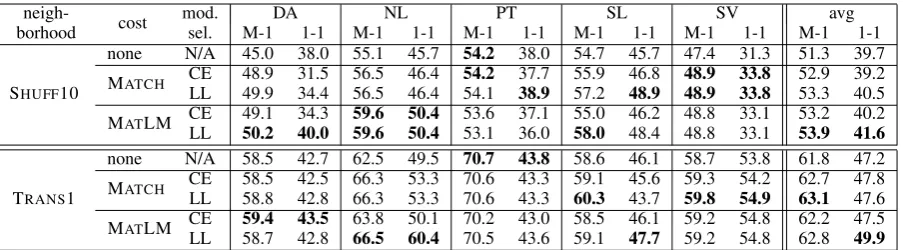
[image:9.595.75.527.61.186.2]none N/A 58.5 42.7 62.5 49.5 70.7 43.8 58.6 46.1 58.7 53.8 61.8 47.2 MATCH CELL 58.558.8 42.542.8 66.366.3 53.353.3 70.670.6 43.343.3 60.359.1 43.745.6 59.859.3 54.954.2 63.162.7 47.847.6 MATLM CELL 59.458.7 43.542.8 63.866.5 50.160.4 70.270.5 43.643.0 59.158.5 47.746.1 59.259.2 54.854.8 62.862.2 47.549.9 Table 2: Results for observation cost functions. The CE baseline corresponds to rows where cost=“none”. Other rows are CCE. Best score for each column and each neighborhood is bold.
Wikipedia. The word counts for the Wikipedias used range from 18M for Slovene to 1.9B for Dutch. We used modified Kneser-Ney smoothing as implemented by SRILM (Stolcke, 2002).
8.2 Results
We present two sets of results. First we compare our MATCH and MATLM observation cost func-tions for our two neighborhoods and two ways of doing model selection. Then we do a broader com-parison, comparing both types of costs and their combination to our full set of baselines.
Observation Cost Functions In Table 2, we show results for observation cost functions. We note that the TRANS1 neighborhood works much better than the SHUFF10 neighborhood, but we find that using cost functions can close the gap in certain cases, particularly for Dutch and Slovene for which the SHUFF10 MATLM scores approach or exceed the TRANS1 scores without a cost.
Since the SHUFF10 neighborhood exhibits more diversity than TRANS1, we expect to see larger gains from using observation cost functions. We do in fact see larger gains in M-1, e.g., average improvements are 1.6-2.6 for SHUFF10 and 0.4-1.3 for TRANS1, though 1-1 gains are closer.
For TRANS1, while MATCH does reach a slightly higher average M-1 than MATLM, the lat-ter does much betlat-ter in 1-1 (49.9 vs. 47.6 when using LL for model selection). For SHUFF10, MATLM consistently does better than MATCH. Nonetheless, we suspect MATCHworks as well as it does because it at least differentiates the obser-vation (which is always part of the neighborhood) from the corruptions.
We find that the LL model selection criterion consistently works better than the CE criterion for model selection. When using LL model selection
and fixing the neighborhood, all average scores are better than their CE baselines. For M-1, the aver-age improvement is 1.0 to 2.6 points, and for 1-1 the average improvement ranges from 0.4 to 2.7.
We find the best overall performance when us-ing MATLM with LL model selection with the TRANS1 neighborhood, and we report this setting in our subsequent experiments.
Output Cost Function Table 3 shows results when using our UNIVoutput cost function, as well as our full set of baselines. All (C)CE experiments used the TRANS1 neighborhood.
We find that our contrastive estimation baseline (cost=“none”) has a higher average M-1 (61.8) than all results from the shared task, but its average 1-1 accuracy is lower than that reached by poste-rior regularization, the best system in the shared task according to 1-1. Using an observation cost function increases both M-1 and 1-1: MATLM yields an average 1-1 of 49.9, nearing the 50.1 of PR while exceeding it in M-1 by nearly 2 points.
When using the UNIV cost function, we see some variation in performance across model selec-tion criteria, but we find improvements in both M-1 and M-1-M-1 accuracy under most settings. When do-ing model selection via ALIGNvoting, we roughly match the average 1-1 of PR, and when using the CE criterion, we beat it by 1 point on average (51.3 vs. 50.1).
system M-1DA1-1 M-1NL1-1 M-1PT1-1 M-1SL1-1 M-1SV1-1 M-1avg1-1 HMM, EM 42.5 28.1 53.0 40.6 59.4 33.7 50.3 34.7 49.3 33.9 50.9 34.2 HMM, stepwise EM 51.7 38.2 61.6 45.2 66.5 46.7 53.6 35.7 55.3 39.6 57.7 41.1 BROWN 47.1 39.2 57.3 43.1 67.6 51.6 58.3 42.3 57.6 51.3 57.6 45.5
mkcls 53.1 44.2 63.0 54.1 68.1 46.3 50.4 40.6 57.3 43.6 58.4 45.8 posterior regularization 53.8 45.6 57.6 45.4 74.4 56.1 60.0 48.5 58.8 54.9 60.9 50.1
contrastive estimation cost model sel.
none N/A 58.5 42.7 62.5 49.5 70.7 43.8 58.6 46.1 58.7 53.8 61.8 47.2 MATCH LL 58.8 42.8 66.3 53.3 70.6 43.3 60.3 43.7 59.8 54.9 63.1 47.6 MATLM LL 58.7 42.8 66.5 60.4 70.5 43.6 59.1 47.7 59.2 54.8 62.8 49.9
UNIV
[image:10.595.83.516.61.278.2]CE 59.7 45.6 60.6 51.1 70.0 62.7 60.9 44.1 57.1 52.8 61.7 51.3 LL 59.5 42.2 62.1 56.3 70.7 43.1 60.9 44.1 57.1 52.8 62.1 47.7 NA¨IVE 59.2 45.6 62.2 52.8 72.7 52.7 60.0 43.8 56.2 53.0 62.2 49.6 ALIGN 61.6 47.3 63.7 54.5 74.4 53.1 59.7 42.1 56.6 53.2 63.2 50.0 MATLM CE 59.8 45.7 60.4 48.4 70.0 62.8 52.9 45.0 59.4 54.9 60.5 51.4 + NALL¨IVE 59.358.5 44.442.5 61.964.9 56.260.3 70.865.4 52.143.1 59.355.5 45.941.9 59.060.0 55.154.4 62.360.6 47.851.4 UNIV ALIGN 61.1 45.4 66.2 60.9 75.8 49.8 59.5 48.2 59.0 54.4 64.3 51.7 Table 3: Unsupervised POS tagging accuracies for five languages, showing results for three systems from the PASCAL shared task as well as three other baselines (EM, stepwise EM, and contrastive estimation). All (C)CE results use the TRANS1 neighborhood. The best score in each column is bold.
we again chose results by CE, LL, and both voting schemes.
The results are shown in the lower part of Ta-ble 3. We find different trends in M-1 and 1-1 depending on whether we use CE or LL for model selection, which may be due to our lim-ited hyperparameter search stemming from com-putational constraints. However, by comparing NA¨IVE to ALIGN, we see a consistent benefit from aligning tags before voting, leading to our highest average accuracies. In particular, using MATCHLM+UNIVand ALIGN, we improve over CE by 2.5 in M-1 and 4.5 in 1-1, also improving over the best results from the shared task.
9 Conclusion
We have shown how to modify contrastive estima-tion to use addiestima-tional sources of knowledge, both in terms of observation and output cost functions. We adapted a recently-proposed technique for es-timating the log-likelihood of held-out data, find-ing it to be effective as a model selection criterion when using observation cost functions. We im-proved tagging accuracy by using weak supervi-sion in the form of universal tag frequencies. We proposed a system combination method for POS induction systems that consistently performs bet-ter than na¨ıve voting and circumvents hyperpa-rameter selection. We reported results on par with or exceeding the best systems from the PASCAL 2012 shared task.
Contrastive estimation has been shown effective for numerous NLP tasks, including dependency grammar induction (Smith and Eisner, 2005b), bilingual part-of-speech induction (Chen et al., 2011), morphological segmentation (Poon et al., 2009), and machine translation (Xiao et al., 2011). The hope is that our contributions can benefit these and other applications of weakly-supervised learn-ing.
Acknowledgments
We thank the anonymous reviewers for their in-sightful comments and Waleed Ammar, Chris Dyer, David McAllester, Sasha Rush, Nathan Schneider, Noah Smith, and John Wieting for helpful discussions.
References
S. Afonso, E. Bick, R. Haber, and D. Santos. 2002. Floresta sint´a(c)tica: a treebank for Portuguese. In
Proc. of LREC.
Y. Bengio, L. Yao, and K. Cho. 2013. Bounding the test log-likelihood of generative models. arXiv preprint arXiv:1311.6184.
T. Berg-Kirkpatrick, A. Bouchard-Cˆot´e, J. DeNero, and D. Klein. 2010. Painless unsupervised learn-ing with features. InProc. of NAACL.
P. Blunsom and T. Cohn. 2011. A hierarchical Pitman-Yor process HMM for unsupervised part of speech induction. InProc. of ACL.
G. Bouma, G. Van Noord, and R. Malouf. 2001. Alpino: Wide-coverage computational analysis of
Dutch. Language and Computers, 37(1).
P. F. Brown, P. V. deSouza, R. L. Mercer, V. J. Della Pietra, and J. C. Lai. 1992. Class-based N-gram
models of natural language. Computational
Lin-guistics, 18(4).
M. Buch-Kromann, J. Wedekind, and J. Elming. 2007. The Copenhagen Danish-English dependency
treebank v. 2.0.
code.google.com/p/copenhagen-dependency-treebank.
S. Buchholz and E. Marsi. 2006. CoNLL-X shared
task on multilingual dependency parsing. InProc.
of CoNLL.
D. Chen, C. Dyer, S. B. Cohen, and N. A. Smith. 2011. Unsupervised bilingual POS tagging with Markov
random fields. In Proc. of the First Workshop on
Unsupervised Learning in NLP.
S. Cohen and N. A. Smith. 2009. Shared logistic nor-mal distributions for soft parameter tying in
unsu-pervised grammar induction. InProc. of NAACL.
S. B. Cohen, D. Das, and N. A. Smith. 2011. Unsu-pervised structure prediction with non-parallel mul-tilingual guidance. InProc. of EMNLP.
M. Creutz and K. Lagus. 2005. Unsupervised
mor-pheme segmentation and morphology induction from text corpora using Morfessor 1.0. Helsinki Univer-sity of Technology.
D. Das and S. Petrov. 2011. Unsupervised part-of-speech tagging with bilingual graph-based projec-tions. InProc. of ACL.
S. Della Pietra, V. Della Pietra, and J. Lafferty. 1997.
Inducing features of random fields. IEEE Trans.
Pattern Anal. Mach. Intell., 19(4).
A. Dempster, N. Laird, and D. Rubin. 1977. Maxi-mum likelihood estimation from incomplete data via
the EM algorithm. Journal of the Royal Statistical
Society B, 39:1–38.
B. Dezs, A. J¨uttner, and P. Kov´acs. 2011. LEMON - an
open source C++ graph template library. Electron.
Notes Theor. Comput. Sci., 264(5).
C. B. Do, Q. Le, C. H. Teo, O. Chapelle, and A. Smola. 2008. Tighter bounds for structured estimation. In
Advances in NIPS.
C. Dyer, J. H. Clark, A. Lavie, and N. A. Smith. 2011. Unsupervised word alignment with arbitrary fea-tures. InProc. of ACL.
T. Erjavec, D. Fiser, S. Krek, and N. Ledinek. 2010. The JOS linguistically tagged corpus of Slovene. In
Proc. of LREC.
K. Ganchev and D. Das. 2013. Cross-lingual discrim-inative learning of sequence models with posterior regularization. InProc. of EMNLP.
K. Ganchev, J. Gillenwater, and B. Taskar. 2009. De-pendency grammar induction via bitext projection constraints. InProc. of ACL.
K. Ganchev, J. V. Grac¸a, J. Gillenwater, and B. Taskar. 2010. Posterior regularization for structured latent
variable models. Journal of Machine Learning
Re-search, 11.
D. Gelling, T. Cohn, P. Blunsom, and J. V. Grac¸a. 2012. The PASCAL challenge on grammar
induc-tion. InProc. of NAACL-HLT Workshop on the
In-duction of Linguistic Structure.
K. Gimpel and N. A. Smith. 2010. Softmax-margin CRFs: Training log-linear models with cost func-tions. InProc. of NAACL.
K. Gimpel and N. A. Smith. 2012. Structured ramp loss minimization for machine translation. InProc. of NAACL.
K. Gimpel. 2012. Discriminative Feature-Rich
Mod-eling for Syntax-Based Machine Translation. Ph.D. thesis, Carnegie Mellon University.
S. Goldwater and T. Griffiths. 2007. A fully Bayesian approach to unsupervised part-of-speech tagging. In
Proc. of ACL.
J. V. Grac¸a, K. Ganchev, L. Coheur, F. Pereira, and B. Taskar. 2011. Controlling complexity in part-of-speech induction. J. Artif. Int. Res., 41(2). A. Haghighi and D. Klein. 2006. Prototype-driven
learning for sequence models. In Proc. of
HLT-NAACL.
M. Johnson. 2007. Why doesn’t EM find good HMM
POS-taggers? InProc. of EMNLP-CoNLL.
J. Kaiser, B. Horvat, and Z. Kacic. 2000. A novel loss function for the overall risk criterion based
discrimi-native training of HMM models. InProc. of ICSLP.
D. Klein and C. D. Manning. 2004. Corpus-based induction of syntactic structure: Models of depen-dency and constituency. InProc. of ACL.
P. Koehn. 2005. Europarl: A parallel corpus for statis-tical machine translation. InProc. of MT Summit. Z. Li, Z. Wang, S. Khudanpur, and J. Eisner. 2010.
Unsupervised discriminative language model train-ing for machine translation ustrain-ing simulated confu-sion sets. InProc. of COLING.
P. Liang and D. Klein. 2009. Online EM for
unsuper-vised models. InProc. of NAACL.
P. Liang, B. Taskar, and D. Klein. 2006. Alignment by
agreement. InProc. of HLT-NAACL.
P. Liang. 2005. Semi-supervised learning for natural language. Master’s thesis, Massachusetts Institute of Technology.
B. Merialdo. 1994. Tagging English text with a proba-bilistic model.Computational Linguistics, 20(2).
T. Naseem, B. Snyder, J. Eisenstein, and R. Barzilay. 2009. Multilingual part-of-speech tagging: Two un-supervised approaches.JAIR, 36.
T. Naseem, H. Chen, R. Barzilay, and M. Johnson. 2010. Using universal linguistic knowledge to guide
grammar induction. InProc. of EMNLP.
J. Nivre, J. Nilsson, and J. Hall. 2006. Talbanken05: A Swedish treebank with phrase structure and depen-dency annotation. InProc. of LREC.
J. Nivre, J. Hall, S. K¨ubler, R. McDonald, J. Nils-son, S. Riedel, and D. Yuret. 2007. The CoNLL
2007 shared task on dependency parsing. InProc.
of CoNLL.
F. J. Och. 1995. Maximum-likelihood-sch¨atzung von wortkategorien mit verfahren der kombina-torischen optimierung. Bachelor’s thesis (Studien-arbeit), Friedrich-Alexander-Universit¨at Erlangen-N¨urnburg, Germany.
S. Petrov, D. Das, and R. McDonald. 2012. A univer-sal part-of-speech tagset. InProc. of LREC.
H. Poon, C. Cherry, and K. Toutanova. 2009. Unsuper-vised morphological segmentation with log-linear
models. InProc. of HLT: NAACL.
D. Povey and P. C. Woodland. 2002. Minimum phone error and I-smoothing for improved discrima-tive training. InProc. of ICASSP.
D. Povey, D. Kanevsky, B. Kingsbury, B. Ramabhad-ran, G. Saon, and K. Visweswariah. 2008. Boosted MMI for model and feature space discriminative training. InProc. of ICASSP.
S. Ravi and K. Knight. 2009. Minimized models for
unsupervised part-of-speech tagging. In Proc. of
ACL.
S. Riezler. 1999. Probabilistic Constraint Logic Pro-gramming. Ph.D. thesis, Universit¨at T¨ubingen.
R. Rosenfeld. 1997. A whole sentence maximum en-tropy language model. InProc. of ASRU.
N. A. Smith and J. Eisner. 2004. Annealing techniques for unsupervised statistical language learning. In
Proc. of ACL.
N. A. Smith and J. Eisner. 2005a. Contrastive estima-tion: Training log-linear models on unlabeled data. InProc. of ACL.
N. A. Smith and J. Eisner. 2005b. Guiding unsuper-vised grammar induction using contrastive
estima-tion. InProc. of IJCAI Workshop on Grammatical
Inference Applications.
N. A. Smith and J. Eisner. 2006. Annealing structural bias in multilingual weighted grammar induction. In
Proc. of COLING-ACL.
D. A. Smith and J. Eisner. 2009. Parser adaptation and projection with quasi-synchronous features. In
Proc. of EMNLP.
B. Snyder, T. Naseem, and R. Barzilay. 2009.
Unsu-pervised multilingual grammar induction. InProc.
of ACL.
V. I. Spitkovsky, H. Alshawi, and D. Jurafsky. 2010a. From Baby Steps to Leapfrog: How “Less is More”
in unsupervised dependency parsing. In Proc. of
NAACL-HLT.
V. I. Spitkovsky, H. Alshawi, D. Jurafsky, and C. D. Manning. 2010b. Viterbi training improves
unsu-pervised dependency parsing. InProc. of CoNLL.
V. I. Spitkovsky, D. Jurafsky, and H. Alshawi. 2010c. Profiting from mark-up: Hyper-text annotations for guided parsing. InProc. of ACL.
V. I. Spitkovsky, H. Alshawi, and D. Jurafsky. 2011a. Lateen EM: Unsupervised training with multiple ob-jectives, applied to dependency grammar induction. InProc. of EMNLP.
V. I. Spitkovsky, H. Alshawi, and D. Jurafsky. 2011b. Punctuation: Making a point in unsupervised depen-dency parsing. InProc. of CoNLL.
V. I. Spitkovsky, H. Alshawi, and D. Jurafsky. 2013. Breaking out of local optima with count transforms and model recombination: A study in grammar in-duction. InProc. of EMNLP.
A. Stolcke. 2002. SRILM—an extensible language modeling toolkit. InProc. of ICSLP.
O. T¨ackstr¨om, D. Das, S. Petrov, R. McDonald, and J. Nivre. 2013. Token and type constraints for cross-lingual part-of-speech tagging. Transactions of the Association for Computational Linguistics, 1. B. Taskar, C. Guestrin, and D. Koller. 2003.
Max-margin Markov networks. InAdvances in NIPS 16.
K. Toutanova and M. Johnson. 2007. A Bayesian LDA-based model for semi-supervised part-of-speech tagging. InAdvances in NIPS.
J. Van Gael, A. Vlachos, and Z. Ghahramani. 2009. The infinite HMM for unsupervised POS tagging. InProc. of EMNLP.
A. Vaswani, A. Pauls, and D. Chiang. 2010. Efficient optimization of an MDL-inspired objective function for unsupervised part-of-speech tagging. InProc. of ACL.
M. Wang and C. D. Manning. 2014. Cross-lingual projected expectation regularization for weakly
su-pervised learning. Transactions of the Association
for Computational Linguistics, 2.