Revisiting Embedding Features for Simple Semi supervised Learning

Revisiting Embedding Features for Simple Semi-supervised Learning

Jiang Guo†_{, Wanxiang Che}†_{, Haifeng Wang}‡_{, Ting Liu}†∗ †_{Research Center for Social Computing and Information Retrieval}

Harbin Institute of Technology, China ‡_{Baidu Inc., Beijing, China}

{jguo, car, tliu}@ir.hit.edu.cn [email protected]

Abstract

Recent work has shown success in us-ing continuous word embeddus-ings learned from unlabeled data as features to improve supervised NLP systems, which is re-garded as a simple semi-supervised

learn-ing mechanism. However,

fundamen-tal problems on effectively incorporating the word embedding features within the framework of linear models remain. In this study, we investigate and analyze three different approaches, including a new

pro-posed distributional prototype approach,

for utilizing the embedding features. The presented approaches can be integrated into most of the classical linear models in NLP. Experiments on the task of named entity recognition show that each of the proposed approaches can better utilize the word embedding features, among which thedistributional prototypeapproach per-forms the best. Moreover, the combination of the approaches provides additive im-provements, outperforming the dense and continuous embedding features by nearly 2 points of F1 score.

1 Introduction

Learning generalized representation of words is an effective way of handling data sparsity caused by high-dimensional lexical features in NLP sys-tems, such as named entity recognition (NER)

and dependency parsing. As a typical

low-dimensional and generalized word representa-tion, Brown clustering of words has been stud-ied for a long time. For example, Liang (2005) and Koo et al. (2008) used the Brown cluster features for semi-supervised learning of various NLP tasks and achieved significant improvements.

∗_{Email correspondence.}

Recent research has focused on a special fam-ily of word representations, named “word embed-dings”. Word embeddings are conventionally de-fined as dense, continuous, and low-dimensional vector representations of words. Word embed-dings can be learned from large-scale unlabeled texts through context-predicting models (e.g., neu-ral network language models) or spectneu-ral methods (e.g., canonical correlation analysis) in an unsu-pervised setting.

Compared with the so-calledone-hot

represen-tation where each word is represented as a sparse vector of the same size of the vocabulary and only one dimension is on, word embedding preserves rich linguistic regularities of words with each di-mension hopefully representing a latent feature. Similar words are expected to be distributed close to one another in the embedding space. Conse-quently, word embeddings can be beneficial for a variety of NLP applications in different ways, among which the most simple and general way is to be fed as features to enhance existing supervised NLP systems.

Previous work has demonstrated effectiveness of the continuous word embedding features in sev-eral tasks such as chunking and NER using

gener-alized linear models (Turian et al., 2010).1

How-ever, there still remain two fundamental problems that should be addressed:

• Are the continuous embedding features fit for

the generalized linear models that are most widely adopted in NLP?

• How can the generalized linear models better

utilize the embedding features?

According to the results provided by Turian et

1_{Generalized linear models refer to the models that} de-scribe the data as a combination of linear basis functions, either directly in the input variables space or through some transformation of the probability distributions (e.g., log-linearmodels).

al. (2010), the embedding features brought signif-icantly less improvement than Brown clustering features. This result is actually not reasonable be-cause the expressing power of word embeddings is theoretically stronger than clustering-based rep-resentations which can be regarded as a kind of

one-hotrepresentation but over a low-dimensional vocabulary (Bengio et al., 2013).

Wang and Manning (2013) showed that linear architectures perform better in high-dimensional discrete feature space than non-linear ones, whereas non-linear architectures are more effec-tive in low-dimensional and continuous feature space. Hence, the previous method that directly uses the continuous word embeddings as features in linear models (CRF) is inappropriate. Word embeddings may be better utilized in the linear modeling framework by smartly transforming the embeddings to some relatively higher dimensional and discrete representations.

Driven by this motivation, we present three

different approaches: binarization (Section 3.2),

clustering(Section 3.3) and a new proposed distri-butional prototypemethod (Section 3.4) for better

incorporating the embeddings features. In the

bi-narizationapproach, we directly binarize the con-tinuous word embeddings by dimension. In the

clustering approach, we cluster words based on their embeddings and use the resulting word

clus-ter features instead. In thedistributional prototype

approach, we derive task-specific features from

word embeddings by utilizing a set of

automati-cally extractedprototypesfor each target label.

We carefully compare and analyze these ap-proaches in the task of NER. Experimental results are promising. With each of the three approaches, we achieve higher performance than directly using the continuous embedding features, among which thedistributional prototypeapproach performs the best. Furthermore, by putting the most effective two of these features together, we finally outper-form the continuous embedding features by nearly 2 points of F1 Score (86.21% vs. 88.11%).

The major contribution of this paper is twofold. (1) We investigate various approaches that can bet-ter utilize word embeddings for semi-supervised

learning. (2) We propose a novel distributional

prototypeapproach that shows the great potential of word embedding features. All the presented ap-proaches can be easily integrated into most of the classical linear NLP models.

2 Semi-supervised Learning with Word Embeddings

Statistical modeling has achieved great success in most NLP tasks. However, there still remain some major unsolved problems and challenges, among which the most widely concerned is the data sparsity problem. Data sparsity in NLP is mainly caused by two factors, namely, the lack of labeled training data and the Zipf distribution of words. On the one hand, large-scale labeled training data are typically difficult to obtain, espe-cially for structure prediction tasks, such as syn-tactic parsing. Therefore, the supervised mod-els can only see limited examples and thus make biased estimation. On the other hand, the nat-ural language words are Zipf distributed, which means that most of the words appear a few times or are completely absent in our texts. For these low-frequency words, the corresponding parame-ters usually cannot be fully trained.

More foundationally, the reason for the above factors lies in the high-dimensional and sparse lex-ical feature representation, which completely ig-nores the similarity between features, especially word features. To overcome this weakness, an ef-fective way is to learn more generalized represen-tations of words by exploiting the numerous un-labeled data, in a semi-supervised manner. After which, the generalized word representations can be used as extra features to facilitate the super-vised systems.

Liang (2005) learned Brown clusters of words (Brown et al., 1992) from unlabeled data and use them as features to promote the supervised NER and Chinese word segmentation. Brown clusters of words can be seen as a generalized word representation distributed in a discrete and low-dimensional vocabulary space. Contextually similar words are grouped in the same cluster. The Brown clustering of words was also adopted in de-pendency parsing (Koo et al., 2008) and POS tag-ging for online conversational text (Owoputi et al., 2013), demonstrating significant improvements.

Recently, another kind of word representation named “word embeddings” has been widely stud-ied (Bengio et al., 2003; Mnih and Hinton, 2008). Using word embeddings, we can evaluate the sim-ilarity of two words straightforward by comput-ing the dot-product of two numerical vectors in the

be distributed close to each other.2

Word embeddings can be useful as input to an NLP model (mostly non-linear) or as additional features to enhance existing systems. Collobert et al. (2011) used word embeddings as input to a deep neural network for multi-task learning. De-spite of the effectiveness, such non-linear models are hard to build and optimize. Besides, these ar-chitectures are often specialized for a certain task and not scalable to general tasks. A simple and more general way is to feed word embeddings as augmented features to an existing supervised sys-tem, which is similar to the semi-supervised learn-ing with Brown clusters.

As discussed in Section 1, Turian et al. (2010) is the pioneering work on using word embedding features for semi-supervised learning. However, their approach cannot fully exploit the potential of word embeddings. We revisit this problem in this study and investigate three different ap-proaches for better utilizing word embeddings in semi-supervised learning.

3 Approaches for Utilizing Embedding Features

3.1 Word Embedding Training

In this paper, we will consider a

context-predicting model, more specifically, theSkip-gram

model (Mikolov et al., 2013a; Mikolov et al., 2013b) for learning word embeddings, since it is much more efficient as well as memory-saving than other approaches.

Let’s denote the embedding matrix to be learned

byCd×N, whereN is the vocabulary size anddis

the dimension of word embeddings. Each column

of C represents the embedding of a word. The

Skip-grammodel takes the current wordwas in-put, and predicts the probability distribution of its context words within a fixed window size.

Con-cretely,wis first mapped to its embeddingvw by

selecting the corresponding column vector of C

(or multiplyingC with theone-hotvector of w).

The probability of its context wordcis then

com-puted using a log-linear function:

P(c|w;θ) = P exp(v>cvw)

c0_∈V exp(vc0>v_w) (1)

whereV is the vocabulary. The parametersθare

vwi,vci forw, c ∈ V andi = 1, ..., d. Then, the 2_{The termsimilarshould be viewed depending on the} spe-cific task.

log-likelihood over the entire training dataset D

can be computed as:

J(θ) = X

(w,c)∈D

logp(c|w;θ) (2)

The model can be trained by maximizingJ(θ).

Here, we suppose that the word embeddings have already been trained from large-scale unla-beled texts. We will introduce various approaches for utilizing the word embeddings as features for semi-supervised learning. The main idea, as in-troduced in Section 1, is to transform the continu-ous word embeddings to some relatively higher di-mensional and discrete representations. The direct use of continuous embeddings as features (Turian et al., 2010) will serve as our baseline setting.

3.2 Binarization of Embeddings

One fairly natural approach for converting the continuous-valued word embeddings to discrete values is binarization by dimension.

Formally, we aim to convert the

continuous-valued embedding matrixCd×N, to another matrix

Md×N which is discrete-valued. There are various

conversion functions. Here, we consider a

sim-ple one. For the ith _{dimension of the word}

em-beddings, we divide the corresponding row vector

Ci into two halves for positive (Ci+) and

nega-tive (Ci−), respectively. The conversion function

is then defined as follows:

Mij =φ(Cij) =

    

U+, if Cij ≥mean(Ci+) B−, if Cij ≤mean(Ci−)

0, otherwise

wheremean(v)is the mean value of vectorv,U+

is a string feature which turns on when the value (Cij) falls into the upper part of the positive list.

Similarly,B−refers to the bottom part of the

neg-ative list. The insight behindφis that we only

con-sider the features with strong opinions (i.e., posi-tive or negaposi-tive) on each dimension and omit the values close to zero.

3.3 Clustering of Embeddings

In this study, we again investigate this ap-proach. Concretely, each word is treated as a sin-gle sample. The batch k-means clustering

algo-rithm (Sculley, 2010) is used,3 _{and each cluster}

is represented as the mean of the embeddings of words assigned to it. Similarities between words and clusters are measured by Euclidean distance.

Moreover, different number of clusters n

con-tain information of different granularities. There-fore, we combine the cluster features of different

ns to better utilize the embeddings.

3.4 Distributional Prototype Features

We propose a novel kind of embedding features, named distributional prototype features for su-pervised models. This is mainly inspired by

prototype-driven learning (Haghighi and Klein, 2006) which was originally introduced as a pri-marily unsupervised approach for sequence

mod-eling. In prototype-driven learning, a few

pro-totypical examples are specified for each target label, which can be treated as an injection of prior knowledge. This sparse prototype informa-tion is then propagated across an unlabeled corpus through distributional similarities.

The basic motivation of the distributional pro-totype features is that similar words are supposed to be tagged with the same label. This hypothesis makes great sense in tasks such as NER and POS

tagging. For example, suppose Michaelis a

pro-totype of the named entity (NE) typePER. Using

the distributional similarity, we could link similar

words to the same prototypes, so the wordDavid

can be linked to Michael because the two words

have high similarity (exceeds a threshold). Using

this link feature, the model will pushDavidcloser

toPER.

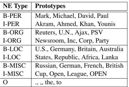
To derive the distributional prototype features, first, we need to construct a few canonical exam-ples (prototypes) for each target annotation label. We use the normalized pointwise mutual informa-tion (NPMI) (Bouma, 2009) between the label and word, which is a smoothing version of the standard PMI, to decide the prototypes of each label. Given the annotated training corpus, the NPMI between a label and word is computed as follows:

λn(label, word) = ₋λ_ln(label, word_{p(label, word}) ₎ (3)

3_{code.google.com/p/sofia-ml}

NE Type Prototypes

B-PER Mark, Michael, David, Paul

I-PER Akram, Ahmed, Khan, Younis

B-ORG Reuters, U.N., Ajax, PSV

I-ORG Newsroom, Inc, Corp, Party

B-LOC U.S., Germany, Britain, Australia

I-LOC States, Republic, Africa, Lanka

B-MISC Russian, German, French, British

I-MISC Cup, Open, League, OPEN

O ., ,, the, to

Table 1: Prototypes extracted from the CoNLL-2003 NER training data using NPMI.

where,

λ(label, word) = ln_pp₍(_labellabel, word_)p(word)₎ (4)

is the standard PMI.

For each target label l (e.g., PER, ORG,LOC),

we compute the NPMI of l and all words in the

vocabulary, and the topmwords are chosen as the

prototypes of l. We should note that the

proto-types are extracted fully automatically, without in-troducing additional human prior knowledge.

Table 1 shows the top four prototypes extracted from the NER training corpus of CoNLL-2003 shared task (Tjong Kim Sang and De Meul-der, 2003), which contains four NE types, namely,

PER,ORG,LOC, andMISC. Non-NEs are denoted

by O. We convert the original annotation to the

standard BIO-style. Thus, the final corpus con-tains nine labels in total.

Next, we introduce the prototypes as features to our supervised model. We denote the set of pro-totypes for all target labels bySp. For each

proto-typez∈Sp, we add a predicateproto=z, which

becomes active at eachwif the distributional

sim-ilarity betweenzandw(DistSim(z, w)) is above

some threshold. DistSim(z, w)can be efficiently

calculated through thecosinesimilarity of the

em-beddings of z andw. Figure 1 gives an

illustra-tion of the distribuillustra-tional prototype features. Un-like previous embedding features or Brown

clus-ters, the distributional prototype features are

task-specific because the prototypes of each label are extracted from the training data.

i -1

x x_i

1



i

y yi

O B-LOC

in /IN

Hague /NNP

O B-LOC

1

( _i, _i) 

f y y

( , )

word = Hague pos = NNP

proto = Britain B-LOC

proto = England ...



 

 

 

 _{ }

 

 

 

 

 

i i

f x y

Figure 1: An example of distributional prototype features for NER.

similar to that prototype are pushed towards that label.

4 Supervised Evaluation Task

Various tasks can be considered to compare and analyze the effectiveness of the above three ap-proaches. In this study, we partly follow Turian et al. (2010) and Yu et al. (2013), and take NER as the supervised evaluation task.

NER identifies and classifies the named entities such as the names of persons, locations, and orga-nizations in text. The state-of-the-art systems typ-ically treat NER as a sequence labeling problem, where each word is tagged either as a BIO-style NE or a non-NE category.

Here, we use the linear chain CRF model, which is most widely used for sequence modeling in the field of NLP. The CoNLL-2003 shared task dataset from the Reuters, which was used by Turian et al. (2010) and Yu et al. (2013), was chosen as our evaluation dataset. The training set contains 14,987 sentences, the development set contains 3,466 sentences and is used for parameter tuning, and the test set contains 3,684 sentences.

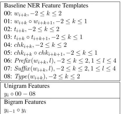
The baseline features are shown in Table 2.

4.1 Embedding Feature Templates

In this section, we introduce the embedding fea-tures to the baseline NER system, turning the su-pervised approach into a semi-susu-pervised one.

Dense embedding features. The dense con-tinuous embedding features can be fed directly to the CRF model. These embedding features can be seen as heterogeneous features from the exist-ing baseline features, which are discrete. There is no effective way for dense embedding features to be combined internally or with other discrete tures. So we only use the unigram embedding fea-tures following Turian et al. (2010). Concretely, the embedding feature template is:

Baseline NER Feature Templates 00:wi+k,−2≤k≤2

01:wi+k◦wi+k+1,−2≤k≤1

02:ti+k,−2≤k≤2

03:ti+k◦ti+k+1,−2≤k≤1

04:chki+k,−2≤k≤2

05:chki+k◦chki+k+1,−2≤k≤1

06:Prefix(wi+k, l),−2≤k≤2,1≤l≤4

07:Suffix(wi+k, l),−2≤k≤2,1≤l≤4

08:Type(wi+k),−2≤k≤2

Unigram Features

yi◦00−08

Bigram Features

yi−1◦yi

Table 2: Features used in the NER system. tis

the POS tag. chk is the chunking tag. Prefix

andSuffix are the first and last l characters of a

word.Type indicates if the word is all-capitalized,

is-capitalized, all-digits, etc.

• dei+k[d], −2 ≤ k ≤ 2, dranges over the

dimensions of the dense word embeddingde.

Binarized embedding features. The binarized embedding feature template is similar to the dense one. The only difference is that the feature val-ues are discrete and we omit dimensions with zero value. Therefore, the feature template becomes:

• bii+k[d],−2 ≤ k ≤ 2, where bii+k[d] 6= 0,

dranges over the dimensions of the binarized

vectorbiof word embedding.

In this way, the dimension of the binarized

em-bedding feature space becomes 2×d compared

with the originallydof the dense embeddings.

Compound cluster features. The advantage of the cluster features is that they can be combined internally or with other features to form compound features, which can be more discriminative.

Fur-thermore, the number of resulting clusters n can

be tuned, and differentns indicate different

granu-larities. Concretely, the compound cluster feature

template for each specificnis:

• ci+k,−2≤k≤2.

• ci+k◦ci+k+1,−2≤k≤1. • ci−1◦ci+1.

Distributional prototype features. The set of

de-cided by selecting the topm(NPMI) words as

pro-totypes of each label, wheremis tuned on the

de-velopment set. For each word wi in a sequence,

we compute the distributional similarity between

wi and each prototype inSp and select the

proto-typeszs thatDistSim(z, w)≥δ. We setδ = 0.5

without manual tuning. The distributional proto-type feature template is then:

• {protoi+k=z|DistSim(wi+k, z)≥δ&z∈

Sp},−2≤k≤2.

We only use the unigram features, since the number of active distributional prototype features varies for different words (positions). Hence, these features cannot be combined effectively.

4.2 Brown Clustering

Brown clustering has achieved great success in

various NLP applications. At most time, it

provides a strong baseline that is difficult to beat (Turian et al., 2010). Consequently, in our study, we conduct comparisons among the embed-ding features and the Brown clustering features, along with further investigations of their combina-tion.

The Brown algorithm is a hierarchical cluster-ing algorithm which optimizes a class-based bi-gram language model defined on the word clus-ters (Brown et al., 1992). The output of the Brown algorithm is a binary tree, where each word is uniquely identified by its path from the root. Thus each word can be represented as a bit-string with a specific length.

Following the setting of Owoputi et al. (2013), we will use the prefix features of hierarchical clus-ters to take advantage of the word similarity in dif-ferent granularities. Concretely, the Brown cluster feature template is:

• bci+k,−2≤k≤2.

• prefix(bci+k, p), p ∈ {2,4,6,...,16}, −2 ≤

k ≤ 2. prefix takes the p-length prefix of the Brown cluster codingbci+k.

5 Experiments

5.1 Experimental Setting

We take the English Wikipedia until August 2012 as our unlabeled data to train the word

embed-dings.4 _{Little pre-processing is conducted for the}

4_{download.wikimedia.org.}

training of word embeddings. We remove para-graphs that contain non-roman characters and all MediaWiki markups. The resulting text is

tok-enized using the Stanford tokenizer,5 _{and every}

word is converted to lowercase. The final dataset contains about 30 million sentences and 1.52 bil-lion words. We use a dictionary that contains

212,779 most common words (frequency≥80) in

the dataset. An efficient open-source

implementa-tion of theSkip-grammodel is adopted.6 _We

ap-ply the negative sampling7 _{method for}

optimiza-tion, and the asynchronous stochastic gradient de-scent algorithm (Asynchronous SGD) for parallel weight updating. In this study, we set the dimen-sion of the word embeddings to 50. Higher di-mension is supposed to bring more improvements in semi-supervised learning, but its comparison is beyond the scope of this paper.

For the cluster features, we tune the number

of clusters n from 500 to 3000 on the

develop-ment set, and finally use the combination ofn =

500,1000,1500,2000,3000, which achieves the

best results. For the distributional prototype fea-tures, we use a fixed number of prototype words

(m) for each target label.mis tuned on the

devel-opment set and is finally set to 40.

We induce 1,000 brown clusters of words, the setting in prior work (Koo et al., 2008; Turian et al., 2010). The training data of brown clustering is the same with that of training word embeddings.

5.2 Results

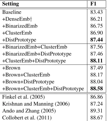
Table 3 shows the performances of NER on the test dataset. Our baseline is slightly lower than that of Turian et al. (2010), because they use the BILOU encoding of NE types which

outper-forms BIO encoding (Ratinov and Roth, 2009).8

Nonetheless, our conclusions hold. As we can see, all of the three approaches we investigate in this study achieve better performance than the direct use of the dense continuous embedding features.

To our surprise, even the binarized embedding features (BinarizedEmb) outperform the continu-ous version (DenseEmb). This provides clear evi-dence that directly using the dense continuous em-beddings as features in CRF indeed cannot fully

5_{nlp.stanford.edu/software/tokenizer.}

shtml.

6_{code.google.com/p/word2vec/.}

Setting F1

Baseline 83.43

+DenseEmb† 86.21

+BinarizedEmb 86.75

+ClusterEmb 86.90

+DistPrototype 87.44

+BinarizedEmb+ClusterEmb 87.56

+BinarizedEmb+DistPrototype 87.46

+ClusterEmb+DistPrototype 88.11

+Brown 87.49

+Brown+ClusterEmb 88.17

+Brown+DistPrototype 88.04

+Brown+ClusterEmb+DistPrototype 88.58

Finkel et al. (2005) 86.86

Krishnan and Manning (2006) 87.24

Ando and Zhang (2005) 89.31

Collobert et al. (2011) 88.67

Table 3: The performance of semi-supervised NER on the CoNLL-2003 test data, using

vari-ous embedding features.†DenseEmb refers to the

method used by Turian et al. (2010), i.e., the direct use of the dense and continuous embeddings.

exploit the potential of word embeddings. The compound cluster features (ClusterEmb) also out-perform the DenseEmb. The same result is also shown in (Yu et al., 2013). Further, the distribu-tional prototype features (DistPrototype) achieve the best performance among the three approaches (1.23% higher than DenseEmb).

We should note that the feature templates used for BinarizedEmb and DistPrototype are merely unigram features. However, for ClusterEmb, we form more complex features by combining the clusters of the context words. We also consider

different number of clustersn, to take advantage

of the different granularities. Consequently, the dimension of the cluster features is much higher than that of BinarizedEmb and DistPrototype.

We further combine the proposed features to see if they are complementary to each other. As shown in Table 3, the cluster and distributional prototype features are the most complementary, whereas the binarized embedding features seem to have large overlap with the distributional prototype features. By combining the cluster and distributional pro-totype features, we further push the performance to 88.11%, which is nearly two points higher than the performance of the dense embedding features

(86.21%).9

We also compare the proposed features with the Brown cluster features. As shown in Table 3, the distributional prototype features alone achieve comparable performance with the Brown clusters. When the cluster and distributional prototype fea-tures are used together, we outperform the Brown clusters. This result is inspiring because we show that the embedding features indeed have stronger expressing power than the Brown clusters, as de-sired. Finally, by combining the Brown cluster features and the proposed embedding features, the performance can be improved further (88.58%). The binarized embedding features are not included in the final compound features because they are al-most overlapped with the distributional prototype features in performance.

We also summarize some of the reported benchmarks that utilize unlabeled data (with no gazetteers used), including the Stanford NER tag-ger (Finkel et al. (2005) and Krishnan and Man-ning (2006)) with distributional similarity fea-tures. Ando and Zhang (2005) use unlabeled data for constructing auxiliary problems that are ex-pected to capture a good feature representation of the target problem. Collobert et al. (2011) adjust the feature embeddings according to the specific task in a deep neural network architecture. We can see that both Ando and Zhang (2005) and

Col-lobert et al. (2011) learntask-specificlexical

fea-tures, which is similar to the proposed

distribu-tional prototypemethod in our study. We suggest this to be the main reason for the superiority of these methods.

Another advantage of the proposed discrete fea-tures over the dense continuous feafea-tures is tag-ging efficiency. Table 4 shows the running time using different kinds of embedding features. We achieve a significant reduction of the tagging time per sentence when using the discrete features. This is mainly due to the dense/sparse battle. Al-though the dense embedding features are low-dimensional, the feature vector for each word is much denser than in the sparse and discrete feature space. Therefore, we actually need much more computation during decoding. Similar results can be observed in the comparison of the DistProto-type and ClusterEmb features, since the density of the DistPrototype features is higher. It is possible

Setting Time (ms) / sent

Baseline 1.04

+DenseEmb 4.75

+BinarizedEmb 1.25

+ClusterEmb 1.16

+DistPrototype 2.31

Table 4: Running time of different features on a Intel(R) Xeon(R) E5620 2.40GHz machine.

to accelerate the DistPrototype, by increasing the

threshold ofDistSim(z, w). However, this is

in-deed an issue of trade-off between efficiency and accuracy.

5.3 Analysis

In this section, we conduct analyses to show the reasons for the improvements.

5.3.1 Rare words

As discussed by Turian et al. (2010), much of the NER F1 is derived from decisions regarding rare words. Therefore, in order to show that the three proposed embedding features have stronger abil-ity for handling rare words, we first conduct anal-ysis for the tagging errors of words with differ-ent frequency in the unlabeled data. We assign the word frequencies to several buckets, and evaluate the per-token errors that occurred in each bucket. Results are shown in Figure 2. In most cases, all three embedding features result in fewer errors on rare words than the direct use of dense continuous embedding features.

Interestingly, we find that for words that are extremely rare (0–256), the binarized embedding features incur significantly fewer errors than other approaches. As we know, the embeddings for the rare words are close to their initial value, because they received few updates during training. Hence, these words are not fully trained. In this case, we would like to omit these features because their embeddings are not even trustable. However, all embedding features that we proposed except Bi-narizedEmb are unable to handle this.

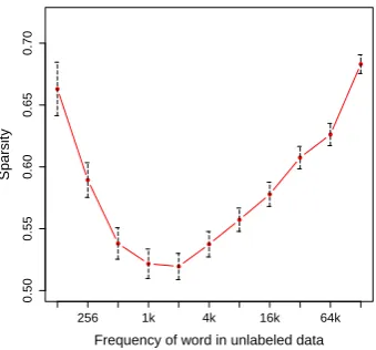
In order to see how much we have utilized the embedding features in BinarizedEmb, we cal-culate the sparsity of the binarized embedding vectors, i.e., the ratio of zero values in each vector (Section 3.2). As demonstrated in Fig-ure 3, the sparsity-frequency curve has good prop-erties: higher sparsity for very rare words and

very frequent words, while lower sparsity for mid-frequent words. It indicates that for words that are very rare or very frequent, BinarizedEmb just omit most of the features. This is reasonable also for the very frequent words, since they usually have rich and diverse context distributions and their embeddings cannot be well learned by our mod-els (Huang et al., 2012).

●

●

●

● ● ●

● ●

● ●

●

Frequency of word in unlabeled data

Sparsity

256 1k 4k 16k 64k

0.50

0.55

0.60

0.65

0.70

Figure 3: Sparsity (with confidence interval) of the binarized embedding vector w.r.t. word frequency in the unlabeled data.

Figure 2(b) further supports our analysis. Bina-rizedEmb also reduce much of the errors for the highly frequent words (32k-64k).

As expected, the distributional prototype fea-tures produce fewest errors in most cases. The

main reason is that the prototype features are

task-specific. The prototypes are extracted from the training data and contained indicative information of the target labels. By contrast, the other em-bedding features are simply derived from general word representations and are not specialized for certain tasks, such as NER.

5.3.2 Linear Separability

Another reason for the superiority of the proposed embedding features is that the high-dimensional discrete features are more linear separable than the low-dimensional continuous embeddings. To verify the hypothesis, we further carry out experi-ments to analyze the linear separability of the pro-posed discrete embedding features against dense continuous embeddings.

respec-0−256 256−512 512−1k 1k−2k

Frequency of word in unlabeled data

n

umber of per−tok

en errors

0

50

100

150

200

250

DenseEmb BinarizedEmb ClusterEmb DistPrototype

(a)

4k−8k 8k−16k 16k−32k 32k−64k

Frequency of word in unlabeled data

n

umber of per−tok

en errors

40

60

80

100

120

DenseEmb BinarizedEmb ClusterEmb DistPrototype

(b)

Figure 2: The number of per-token errors w.r.t. word frequency in the unlabeled data. (a) For rare words

(frequency≤2k). (b) For frequent words (frequency≥4k).

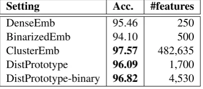
Setting Acc. #features

DenseEmb 95.46 250

BinarizedEmb 94.10 500

ClusterEmb 97.57 482,635

DistPrototype 96.09 1,700

DistPrototype-binary 96.82 4,530

Table 5: Performance of the NE/non-NE classi-fication on the CoNLL-2003 development dataset using different embedding features.

tively. We use the LIBLINEAR tool (Fan et al., 2008) as our SVM implementation. The penalty

parameterCis tuned from 0.1 to 1.0 on the

devel-opment dataset. The results are shown in Table 5. As we can see, NEs and non-NEs can be better separated using ClusterEmb or DistPrototype fea-tures. However, the BinarizedEmb features per-form worse than the direct use of word embedding features. The reason might be inferred from the third column of Table 5. As demonstrated in Wang and Manning (2013), linear models are more ef-fective in high-dimensional and discrete feature space. The dimension of the BinarizedEmb fea-tures remains small (500), which is merely twice the DenseEmb. By contrast, feature dimensions are much higher for ClusterEmb and DistProto-type, leading to better linear separability and thus can be better utilized by linear models.

We notice that the DistPrototype features per-form significantly worse than ClusterEmb in NE identification. As described in Section 3.4, in previous experiments, we automatically extracted prototypes for each label, and propagated the

in-formation via distributional similarities. Intu-itively, the prototypes we used should be more ef-fective in determining fine-grained NE types than identifying whether a word is an NE. To verify this, we extract new prototypes considering only two labels, namely, NE and non-NE, using the same metric in Section 3.4. As shown in the last row of Table 5, higher performance is achieved.

6 Related Studies

Semi-supervised learning with generalized word representations is a simple and general way of im-proving supervised NLP systems. One common approach for inducing generalized word represen-tations is to use clustering (e.g., Brown clustering) (Miller et al., 2004; Liang, 2005; Koo et al., 2008; Huang and Yates, 2009).

Aside from word clustering, word embeddings have been widely studied. Bengio et al. (2003) propose a feed-forward neural network based lan-guage model (NNLM), which uses an embedding layer to map each word to a dense continuous-valued and low-dimensional vector (parameters), and then use these vectors as the input to predict the probability distribution of the next word. The NNLM can be seen as a joint learning framework for language modeling and word representations.

Skip-gram model (Mikolov et al., 2013a; Mikolov et al., 2013b).

Aside from the NNLMs, word embeddings can also be induced using spectral methods, such as latent semantic analysis and canonical correlation analysis (Dhillon et al., 2011). The spectral meth-ods are generally faster but much more memory-consuming than NNLMs.

There has been a plenty of work that exploits word embeddings as features for semi-supervised learning, most of which take the continuous fea-tures directly in linear models (Turian et al., 2010; Guo et al., 2014). Yu et al. (2013) propose com-pound k-means cluster features based on word em-beddings. They show that the high-dimensional discrete cluster features can be better utilized by linear models such as CRF. Wu et al. (2013) fur-ther apply the cluster features to transition-based dependency parsing.

7 Conclusion and Future Work

This paper revisits the problem of semi-supervised learning with word embeddings. We present three different approaches for a careful comparison and analysis. Using any of the three embedding fea-tures, we obtain higher performance than the di-rect use of continuous embeddings, among which the distributional prototype features perform the best, showing the great potential of word embed-dings. Moreover, the combination of the proposed embedding features provides significant additive improvements.

We give detailed analysis about the experimen-tal results. Analysis on rare words and linear sep-arability provides convincing explanations for the performance of the embedding features.

For future work, we are exploring a novel and a theoretically more sounding approach of introduc-ing embeddintroduc-ing kernel into the linear models.

Acknowledgments

We are grateful to Mo Yu for the fruitful discus-sion on the implementation of the cluster-based embedding features. We also thank Ruiji Fu, Meishan Zhang, Sendong Zhao and the anony-mous reviewers for their insightful comments and suggestions. This work was supported by the National Key Basic Research Program of China via grant 2014CB340503 and the National Natu-ral Science Foundation of China (NSFC) via grant 61133012 and 61370164.

References

Rie Kubota Ando and Tong Zhang. 2005. A high-performance semi-supervised learning method for

text chunking. In Proceedings of the 43rd annual

meeting on association for computational linguis-tics, pages 1–9. Association for Computational Lin-guistics.

Yoshua Bengio, R. E. Jean Ducharme, Pascal Vincent, and Christian Janvin. 2003. A neural probabilistic

language model. The Journal of Machine Learning

Research, 3(Feb):1137–1155.

Yoshua Bengio, Aaron Courville, and Pascal Vincent. 2013. Representation learning: A review and new perspectives. Pattern Analysis and Machine Intelli-gence, IEEE Transactions on, 35(8):1798–1828.

Gerlof Bouma. 2009. Normalized (pointwise) mutual

information in collocation extraction. Proceedings

of GSCL, pages 31–40.

Peter F Brown, Peter V Desouza, Robert L Mercer, Vincent J Della Pietra, and Jenifer C Lai. 1992. Class-based n-gram models of natural language.

Computational linguistics, 18(4):467–479.

Ronan Collobert, Jason Weston, L. E. On Bottou, Michael Karlen, Koray Kavukcuoglu, and Pavel Kuksa. 2011. Natural language processing (almost)

from scratch. The Journal of Machine Learning

Re-search, 12:2493–2537.

Paramveer S. Dhillon, Dean P. Foster, and Lyle H. Un-gar. 2011. Multi-view learning of word embeddings

via cca. InNIPS, volume 24 ofNIPS, pages 199–

207.

Rong-En Fan, Kai-Wei Chang, Cho-Jui Hsieh, Xiang-Rui Wang, and Chih-Jen Lin. 2008. Liblinear: A library for large linear classification. The Journal of Machine Learning Research, 9:1871–1874.

Jenny Rose Finkel, Trond Grenager, and Christopher Manning. 2005. Incorporating non-local informa-tion into informainforma-tion extracinforma-tion systems by gibbs

sampling. InProceedings of the 43rd Annual

Meet-ing on Association for Computational LMeet-inguistics, pages 363–370. Association for Computational Lin-guistics.

Yoav Goldberg and Omer Levy. 2014. word2vec ex-plained: deriving mikolov et al.’s negative-sampling

word-embedding method. CoRR, abs/1402.3722.

Jiang Guo, Wanxiang Che, Haifeng Wang, and Ting Liu. 2014. Learning sense-specific word

embed-dings by exploiting bilingual resources. In

Aria Haghighi and Dan Klein. 2006. Prototype-driven

learning for sequence models. In Proceedings of

the main conference on Human Language Technol-ogy Conference of the North American Chapter of the Association of Computational Linguistics, pages 320–327. Association for Computational Linguis-tics.

Fei Huang and Alexander Yates. 2009. Distribu-tional representations for handling sparsity in super-vised sequence-labeling. InProceedings of the Joint Conference of the 47th Annual Meeting of the ACL and the 4th International Joint Conference on Natu-ral Language Processing of the AFNLP: Volume 1-Volume 1, Proceedings of the Joint Conference of the 47th Annual Meeting of the ACL and the 4th Inter-national Joint Conference on Natural Language Pro-cessing of the AFNLP: Volume 1-Volume 1, pages 495–503.

Eric H. Huang, Richard Socher, Christopher D. Man-ning, and Andrew Y. Ng. 2012. Improving word representations via global context and multiple word

prototypes. InProc. of the Annual Meeting of the

Association for Computational Linguistics (ACL), Proc. of the Annual Meeting of the Association for Computational Linguistics (ACL), pages 873–882, Jeju Island, Korea. ACL.

Terry Koo, Xavier Carreras, and Michael Collins. 2008. Simple semi-supervised dependency pars-ing. In Kathleen McKeown, Johanna D. Moore, Si-mone Teufel, James Allan, and Sadaoki Furui,

edi-tors,Proc. of ACL-08: HLT, Proc. of ACL-08: HLT,

pages 595–603, Columbus, Ohio. ACL.

Vijay Krishnan and Christopher D Manning. 2006. An effective two-stage model for exploiting non-local dependencies in named entity recognition. In

Proceedings of the 21st International Conference on Computational Linguistics and the 44th annual meeting of the Association for Computational Lin-guistics, pages 1121–1128. Association for Compu-tational Linguistics.

Percy Liang. 2005.Semi-supervised learning for natu-ral language. Master thesis, Massachusetts Institute of Technology.

Tomas Mikolov, Kai Chen, Greg Corrado, and Jeffrey Dean. 2013a. Efficient estimation of word repre-sentations in vector space. InProc. of Workshop at

ICLR, Proc. of Workshop at ICLR, Arizona.

Tomas Mikolov, Ilya Sutskever, Kai Chen, Greg S. Cor-rado, and Jeff Dean. 2013b. Distributed representa-tions of words and phrases and their compositional-ity. In Proc. of the NIPS, Proc. of the NIPS, pages 3111–3119, Nevada. MIT Press.

Tomas Mikolov. 2012. Statistical Language Models

Based on Neural Networks. Ph. d. thesis, Brno Uni-versity of Technology.

Scott Miller, Jethran Guinness, and Alex Zamanian. 2004. Name tagging with word clusters and

discrim-inative training. In HLT-NAACL, volume 4, pages

337–342.

Andriy Mnih and Geoffrey E. Hinton. 2008. A scal-able hierarchical distributed language model. In

Proc. of the NIPS, Proc. of the NIPS, pages 1081– 1088, Vancouver. MIT Press.

Olutobi Owoputi, Brendan O’Connor, Chris Dyer, Kevin Gimpel, Nathan Schneider, and Noah A Smith. 2013. Improved part-of-speech tagging for online conversational text with word clusters. In

Proceedings of NAACL-HLT, pages 380–390. Lev Ratinov and Dan Roth. 2009. Design challenges

and misconceptions in named entity recognition. In

Proceedings of the Thirteenth Conference on Com-putational Natural Language Learning, CoNLL ’09, pages 147–155, Stroudsburg, PA, USA. Association for Computational Linguistics.

D Sculley. 2010. Combined regression and ranking. In Proceedings of the 16th ACM SIGKDD interna-tional conference on Knowledge discovery and data mining, pages 979–988. ACM.

Erik F Tjong Kim Sang and Fien De Meulder. 2003. Introduction to the conll-2003 shared task: Language-independent named entity recognition. In

Proceedings of the seventh conference on Natural language learning at HLT-NAACL 2003-Volume 4, pages 142–147. Association for Computational Lin-guistics.

Joseph Turian, Lev Ratinov, and Yoshua Bengio. 2010. Word representations: a simple and general method for semi-supervised learning. In Jan Hajic,

San-dra Carberry, and Stephen Clark, editors, Proc. of

the Annual Meeting of the Association for Computa-tional Linguistics (ACL), Proc. of the Annual Meet-ing of the Association for Computational LMeet-inguistics (ACL), pages 384–394, Uppsala, Sweden. ACL. Mengqiu Wang and Christopher D. Manning. 2013.

Effect of non-linear deep architecture in sequence la-beling. InProc. of the Sixth International Joint Con-ference on Natural Language Processing, Proc. of the Sixth International Joint Conference on Natural Language Processing, pages 1285–1291, Nagoya, Japan. Asian Federation of Natural Language Pro-cessing.

Xianchao Wu, Jie Zhou, Yu Sun, Zhanyi Liu, Dian-hai Yu, Hua Wu, and Haifeng Wang. 2013. Gener-alization of words for chinese dependency parsing.

IWPT-2013, page 73.

Mo Yu, Tiejun Zhao, Daxiang Dong, Hao Tian, and Di-anhai Yu. 2013. Compound embedding features for

semi-supervised learning. InProc. of the

NAACL-HLT, Proc. of the NAACL-HLT, pages 563–568,