Training Continuous Space Language Models: Some Practical Issues

Training continuous space language models:

some practical issues

Le Hai Son and Alexandre Allauzen and Guillaume Wisniewski and Franc¸ois Yvon Univ. Paris-Sud, France and LIMSI/CNRS

BP 133, 91403 Orsay Cedex [email protected]

Abstract

Using multi-layer neural networks to esti-mate the probabilities of word sequences is a promising research area in statistical lan-guage modeling, with applications in speech recognition and statistical machine transla-tion. However, training such models for large vocabulary tasks is computationally challeng-ing which does not scale easily to the huge corpora that are nowadays available. In this work, we study the performance and behav-ior of two neural statistical language models so as to highlight some important caveats of the classical training algorithms. The induced word embeddings for extreme cases are also analysed, thus providing insight into the con-vergence issues. A new initialization scheme and new training techniques are then intro-duced. These methods are shown to greatly re-duce the training time and to significantly im-prove performance, both in terms of perplexity and on a large-scale translation task.

1 Introduction

Statistical language models play an important role in many practical applications, such as machine trans-lation and automatic speech recognition. Let V be a finite vocabulary, statistical language models de-fine distributions over sequences of wordswL₁ inV? usually factorized as:

P(w₁L) =P(w1) L

Y

l=1

P(wl|wl1−1)

Modeling the joint distribution of several discrete random variables (such as words in a sentence) is

difficult, especially in real-world Natural Language Processing applications whereV typically contains dozens of thousands words.

Many approaches to this problem have been pro-posed over the last decades, the most widely used being back-off n-gram language models. n-gram models rely on a Markovian assumption, and de-spite this simplification, the maximum likelihood es-timate (MLE) remains unreliable and tends to under-estimate the probability of very raren-grams, which are hardly observed even in huge corpora. Con-ventional smoothing techniques, such as Kneser-Ney and Witten-Bell back-off schemes (see (Chen and Goodman, 1996) for an empirical overview, and (Teh, 2006) for a Bayesian interpretation), per-form back-off on lower order distributions to pro-vide an estimate for the probability of these unseen events. n-gram language models rely on a discrete space representation of the vocabulary, where each word is associated with a discrete index. In this model, the morphological, syntactic and semantic relationships which structure the lexicon are com-pletely ignored, which negatively impact the gen-eralization performance of the model. Various ap-proaches have proposed to overcome this limita-tion, notably the use of word-classes (Brown et al., 1992; Niesler, 1997), of generalized back-off strate-gies (Bilmes et al., 1997) or the explicit integration of morphological information in the random-forest model (Xu and Jelinek, 2004; Oparin et al., 2008).

One of the most successful alternative to date is to usedistributed word representations(Bengio et al., 2003), where distributionally similar words are rep-resented as neighbors in a continuous space. This

turns n-grams distributions into smooth functions of the word representations. These representations and the associated probability estimates are jointly computed in a multi-layer neural network architec-ture. This approach has showed significant and consistent improvements when applied to automatic speech recognition (Schwenk, 2007; Emami and Mangu, 2007; Kuo et al., 2010) and machine trans-lation tasks (Schwenk et al., 2006). Hence, contin-uous space language models are becoming increas-ingly used. These successes have revitalized the re-search on neuronal architectures for language mod-els, and given rise to several new proposals (see, for instance, (Mnih and Hinton, 2007; Mnih and Hinton, 2008; Collobert and Weston, 2008)). A major diffi-culty with these approaches remains the complexity of training, which does not scale well to the mas-sive corpora that are nowadays available. Practical solutions to this problem are discussed in (Schwenk, 2007), which introduces a number of optimization and tricks to make training doable. Even then, train-ing a neuronal language model typically takes days. In this paper, we empirically study the conver-gence behavior of two multi-layer neural networks for statistical language modeling, comparing the standard model of (Bengio et al., 2003) with the log-bilinear (LBL) model of (Mnih and Hinton, 2007). Our contributions are the following: we first pro-pose a reformulation of Mnih and Hinton’s model, which reveals its similarity with extant models, and allows a direct and fair comparison with the stan-dard model. For the stanstan-dard model, these results highlight the impact of parameter initialization. We first investigate a re-initialization method which al-lows to escape from the local extremum the standard model converges to. While this method yields a sig-nificative improvement, the underlying assumption about the structure of the model does not meet the requirement of very large-scale tasks. We therefore introduce a different initialization strategy, called

one vector initialization. Experimental results show that these novel training strategies drastically reduce the total training time, while delivering significant improvements both in terms of perplexity and in a large-scale translation task.

The rest of this paper is organized as follows. We first describe, in Section 2, the standard and the LBL language models. By reformulating the latter, we

show that both models are very similar and empha-size the remaining differences. Section 2.4 discusses complexity issues and possible solutions to reduce the training time. We then report, in Section 3, pre-liminary experimental results that enlighten some caveats of the standard approach. Based on these observations, we introduce in Section 4 novel and more efficient training schemes, yielding improved performance and a reduced training time both on small and large scale experiments.

2 Continuous space language models

Learning a language model amounts to estimate the parameters of the discrete conditional distribution over words given each possible history, where the history corresponds to some function of the preced-ing words. For an n-gram model, the history con-tains the n − 1 preceding words, and the model parameters correspond toP(wl|w_ll−−n+11 ). Continu-ous space language models aim at computing these estimates based on a distributed representation of words (Bengio et al., 2003), thereby reducing the sparsity issues that plague conventional maximum likelihood estimation. In this approach, each word in the vocabulary is mapped into a real-valued vec-tor and the conditional probability distributions are then expressed as a (parameterized) smooth func-tion of these feature vectors. The formalism of neu-ral networks allows to express these two steps in a well-known framework, where, crucially, the map-ping and the model parameters can be learned in conjunction. In the next paragraphs, we describe the two continuous space language models considered in our study and present the various issues associ-ated with the training of such models, as well as their most common remedies.

2.1 The standard model

In the following, we will consider words as indices in a finite dictionary of size V; depending on the context,wwill either refer to the word or to its in-dex in the dictionary. A wordwcan also be repre-sented by a 1-of-V coding vectorvofRV in which

as its output. It consists of three layers.

The first layer builds a continuous representation of the history by mapping each word into its real-valued representation. This mapping is defined by

RTv, where R ∈ RV×m is a projection matrix

andmis the dimension of the continuous projection word space. The output of this layer is a vectoriof

(n−1)m real numbers obtained by concatenating the representations of the context words. The pro-jection matrixRis shared along all positions in the history vector and is learned automatically.

The second layer introduces a non-linear trans-form, where the output layer activation values are defined byh = tanh (Wihi+bih),whereiis the input vector,Wih ∈RH×(n−1)mandbih ∈RH are

the parameters of this layer. The vectorh∈_RH_can be considered as an higher (more abstract) represen-tation of the context thani.

The third layer is an output layer that estimates the desired probability, thanks to thesoftmaxfunction:

P(wl=k|wl_l−−1n+1) =

exp(ok)

P

k0exp(o_k0) (1) o = Whoh+bho, (2)

where Who ∈ RV×H andbho ∈ RV are

respec-tively the projection matrix and the bias term associ-ated with this layer. Thewth_{component inP}

corre-sponds to the estimated probability of thewth word of the vocabulary given the input history vector.

The standard model has two hyper-parameters (the dimension of projection spacemand the size of hidden layer, H) that define the architecture of the neural network and a set of free parametersΘthat need to be learned from data: the projection matrix

R, the weight matrixWih, the bias vectorbih, the weight matrixWhoand the bias vectorbho.

In this model, the projection matricesRandWho play similar roles as they define maps between the vocabulary and the hidden representation. The fact that R assigns similar representations to history words w1 and w2 implies that these words can be exchanged with little impact on the resulting prob-ability distribution. Likewise, the similarity of two lines inWhois an indication that the corresponding words tend to have a similar behavior, i.e. tend to have a similar probabilities of occurrence in all con-texts. In the remainder, we will therefore refer toR

as the matrix representing thecontext space, and to

Who as the matrix for theprediction space.

2.2 The log-bilinear model

The work reported (Mnih and Hinton, 2007) de-scribes another parameterization of the architecture introduced in the previous section. This parameter-ization is based on Factored Restricted Boltzmann Machine. According to (Mnih and Hinton, 2007), this model, termed thelog-bilinearlanguage model (LBL), achieves, for large vocabulary tasks, bet-ter results in bet-terms of perplexity than the standard model, even if the reasons beyond this improvement remain unclear.

In this section, we will describe this model and show how it relates to the standard model. The LBL model estimates then-gram parameters by:

P(wl|w_ll−−1n+1) =

exp(−E(wl;wll−−n+11 ))

P

wexp(−E(w;w l−1 l−n+1))

(3)

In this equation,Eis anenergy functiondefined as:

E(wl;wl1−1) =−

l−1

X

k=l−n+1

vkTRCTk

!

RTvl

(4)

−brTRTvl−bvTvl

=−vT_l R

l−1

X

k=l−n+1

CkRTvk+br

!

−v_lTbv (5)

whereRis the projection matrix introduced above,

(vk)l−n+1≤k≤l−1 are the 1-of-V coding vectors for the history words andvlis the coding vector forwl;

Ck ∈Rm×mis a combination matrix andbrandbv denote bias vectors. All these parameters need to be learned during training.

Equation (4) can be rewritten using the notations introduced for the standard model. We then rename

brandbvrespectivelybihandbho. We also denote

and (3) can be rewritten as:

h=Wihi+bih

o=Rh+bho

P(wl=k|wll−−n+11 ) =

exp(ok)

P

k0exp(o_k0)

This formulation allows to highlight the similarity of the LBL model and the standard model. These two models differ only by the activation function of their hidden layer (linear for the LBL model and tangent hyperbolic for the standard model) and by their def-inition of the prediction space: for the LBL model, the context space and the prediction space are the same (R = Who, and thusH = m), while in the standard model, the prediction space is defined in-dependently from the context space. This restriction drastically reduces the number of free parameters of the LBL model.

It is finally noteworthy to outline the similarity of this model with standard maximum entropy lan-guage models (Lau et al., 1993; Rosenfeld, 1996). Letx denote the binary vector formed by stacking the (n-1) 1-of-V encodings of the history words; then the conditional probability distributions esti-mated in the model are proportional to expF(x), whereF is an affine transform ofx. The main dif-ference with MaxEnt language models are thus the restricted form of the feature functions, which only test one history word, and the particular representa-tion ofF, which is defined as:

F(x) =RWihR0 T

v+Rbih+bho

where, as before, R0 is formed by concatenating

(n−1)copies of the projection matrixR.

2.3 Training and inference

Training the two models introduced above can be achieved by maximizing the log-likelihoodLof the parameters Θ. This optimization is usually per-formed by stochastic back-propagation as in (Ben-gio et al., 2003). For all our experiments, the learn-ing rate is fixed at5×10−3. The learning weight de-cay and the the weight dede-cay (respectively1×10−9 and0) seem to have a minor impact on the results. Learning starts with a random initialization of the

parameters under the uniform distribution and con-verges to a local maximum of the log-likelihood function. Moreover, to prevent overfitting, an early stopping strategy is adopted: after each epoch, train-ing is stopped when the likelihood of a validation set stops increasing.

2.4 Complexity issues

The main problem with neural language models is their computational complexity. For the two mod-els presented in this section, the number of floating point operations needed to predict the label of a sin-gle example is1:

((n−1)·m+ 1)×H+ (H+ 1)×V (6)

where the first term of the sum corresponds to the computation of the hidden layer and the second one to the computation of the output layer. The projec-tion of the context words amounts to select one row of the projection matrixR, as the words are repre-sented with a 1-of-V coding vector. We can there-fore assume that the computation complexity of the first layer is negligible. Most of the computation time is thus spent in the output layer, which implies that the computing time grows linearly with the vo-cabulary size. Training these models for large scale tasks is therefore challenging, and a number of tricks have been introduced to make training and inference tractable (Schwenk and Gauvain, 2002; Schwenk, 2007).

Short list A simple method to reduce the com-plexity in inference and in learning is to reduce the size of the output vocabulary (Schwenk, 2007): rather than estimating the probability P(wl = w|w_ll₋−1_n+1)for all words in the vocabulary, we only estimate it for the N most frequent words of the training set (the so-called short-list). In this case, two vocabularies need to be considered, correspond-ing respectively to thecontext vocabularyV_cused to define the history; and theprediction vocabularyVp. However, this method fails to deliver any probability estimate for words outside of the prediction vocab-ulary, meaning that a fall-back strategy needs to be defined for those words. In practice, neural network

1

language models are combined with a conventional n-gram model as described in (Schwenk, 2007).

Batch mode and resampling Additional speed-ups can be obtained by propagating several exam-ples at once through the network (Bilmes et al., 1997). This “batch mode” allows to factorize the matrix operations and cut down both inference and training time. In all our experiments, we used a batch size of 64. Moreover, the training time is lin-ear in the number of examples in the training data2. Training on very large corpora, which, nowadays, comprise billions of word tokens, cannot be per-formed exhaustively and requires to adopt resam-plingstrategies, whereby, at each epoch, the system is trained with only a small random subset of the training data. This approach enables to effectively estimate neural language models on very large cor-pora; it has also been observed empirically that sam-pling the training data can increase the generaliza-tion performance (Schwenk, 2007).

3 A head-to-head comparison

In this section, we analyze a first experimental study of the two neural network language models introduced in Section 2 in order to better under-stand the differences between these models espe-cially in terms of the word representations they in-duce. Based on this study, we will propose, in the next section, improvements of both the speed and the prediction capacity of the models. In all our ex-periments,4-gram language models are used.

3.1 Corpus

The data we use for training is a large monolingual corpus, containing all the English texts in the par-allel data of the Arabic to English NIST 2009 con-strained task3. It consists of176millions word to-kens with532,557different word types as the size of vocabulary. The perplexity is computed with re-spect to the 2006 NIST test data, which is used here as our development data.

2

Equation (6) gives the complexity of inference for a single example.

3

http://www.itl.nist.gov/iad/mig/tests/ mt/2009/MT09_ConstrainedResources.pdf

3.2 Convergence study

In a first experiment, we trained the two models in the same setting: we choose to consider a small vocabulary comprising the 10,000 most frequent words. The same vocabulary is used to constrain the words occurring in the history and the words to be predicted. The size of hidden layer is set to m=H = 200, the history contains the3preceding words, we use a batch size of 64, a resampling rate of5%and no weight decay.

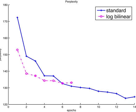
Figure 1 displays the perplexity convergence curve measured on the development data for the standard and the LBL models4. The convergence perplexities after the combination with the standard back-off model are also provided for all the mod-els in table 2 (see section 4.3). We can observe that the LBL model converges faster than the stan-dard model: the latter needs 13 epochs to reach the stopping criteria, while the former only needs 6 epochs. However, upon convergence, the stan-dard model reaches a lower perplexity than the LBL model.

0 2 4 6 8 10 12 14

120 130 140 150 160 170 180

epochs

perplexity

Perplexity

standard log bilinear

Figure 1: Convergence rate of the standard and the LBL models evaluated by the evolution of the perplexity on a development set

As described in Section 2.2, the main difference between the standard and the LBL model is the way the context and the prediction spaces are defined: in the standard model, the two spaces are distinct; in

4_{The use of a back-off4-model estimated with the modified}

the LBL model, they are bound to be the same. With a smaller number of parameters, the LBL model can not capture as many characteristics of the data as the standard model, but it converges faster5. This differ-ence in convergdiffer-ence can be explained by the scarcity of the updates in the projection matrix R in the standard model: during backpropagation, only those weights that are associated with words in the history are updated. By contrast, each training sample up-dates all the weights in the prediction matrixWho.

3.3 An analysis of the continuous word space

To deepen our understanding, we propose to further analyze the induced word embeddings by finding, for some randomly selected words, the five nearest neighbors (according to the Euclidian distance) in the context space and in the prediction space of the two models. Results are presented in Table 1.

If we look first at the standard model, the global picture is that for frequent words (is, are, and, to a lesser extend, have), both spaces seem to define meaningful neighborhood, corresponding to seman-tic and syntacseman-tic similarities; this is less true for rarer words, where we see a greater discrepancy between the context and prediction spaces. For instance, the date 1947 seems to be randomly associated in the context space, while the 5 nearest words in the pre-diction space form a consistent set of dates. The same trend is also observed for the wordCastro. Our interpretation is that for less frequent words, the pro-jection vectors are hardly ever updated and remain close to their original random initialization.

By contrast, the similarities in the (unique) pro-jection space of the LBL remain consistent for all frequency ranges, and are very similar to the predic-tion space of the standard model. This seems to val-idate our hypothesis that in the standard model, the prediction space is learned much faster than the con-text space and corroborates our interpretation of the impact of the scarce updates of rare words. Another possible explanation is that there is no clear relation

5

We could increase the number of parameters of the LBL model for a fairer comparison with the standard model. How-ever, this would also increase the size of the vocabulary and cause two new issues: on one hand, the time complexity would drastically increase for the LBL model, and on the other hand, both models would not be comparable in terms of perplexity as their vocabulary would be different.

between the context space and the target function: the context space is learned only indirectly by back-propagation. As a result, due to the random initial-ization of the parameters and to data sparsity, many vectors ofRmight be blocked in some local max-ima, meaning that similar vectors cannot be grouped in a consistent way and that the induced similarity is more “loose”.

4 Improving the standard model

In Section 3.2, we observed that slightly better re-sults can be obtained with the standard rather than with the LBL model. The latter is however much faster to train, and seems to induce better projection matrices. Both effects can be attributed to the partic-ular parameterization of this model, which uses the same projection matrix both for the context and for the prediction spaces. In this section, we propose several new learning regimes that allowed us to im-prove the standard model in terms of both speed and prediction capacity. All these improvements rely on the idea of sharing word representations. While this idea is not new (see for instance (Collobert and We-ston, 2008)), our analysis enables to better under-stand its impact on the convergence rate. Finally, the improvements we propose are evaluated on a real-word machine translation task.

4.1 Improving performances with re-initialization

The experiments reported in the previous section suggest that it is possible to improve the perfor-mances of the standard model by building a better context space. Thus, we introduce a new learning regime, called re-initialization which aims to im-prove the context space by re-injecting the informa-tion on word neighborhoods that emerges in the pre-diction space. One possible implementation of this idea is as follows:

1. train a standard model until convergence;

2. use the prediction space of this model to ini-tialize the context space of a new model; the prediction space is chosen randomly;

Table 1: The 5 closest words in the representation spaces of the standard and LBL language models.

word (frequency) model space 5 most closest words

is standard context was are were be been 900,350 standard prediction was has would had will

LBL both was reveals proves are ON are standard context were is was be been 478,440 standard prediction were could will have can

LBL both were is was FOR ON have standard context had has of also the 465,417 standard prediction are were provide remain will

LBL both had has Have were embrace meeting standard context meetings conference them 10 talks 150,317 standard prediction undertaking seminar meetings gathering project

LBL both meetings summit gathering festival hearing Imam standard context PCN rebellion 116. Cuba 49 787 standard prediction Castro Sen Nacional Al- Ross

LBL both Salah Khaled Al- Muhammad Khalid 1947 standard context 36 Mercosur definite 2002-2003 era 774 standard prediction 1965 1945 1968 1964 1975

LBL both 1965 1976 1964 1968 1975 Castro standard context exclusively 12. Boucher Zeng Kelly 768 standard prediction Singh Clark da Obasanjo Ross

LBL both Clark Singh Sabri Rafsanjani Sen

Figure 2: Evolution of the perplexity on a development set for various initialization regimes.

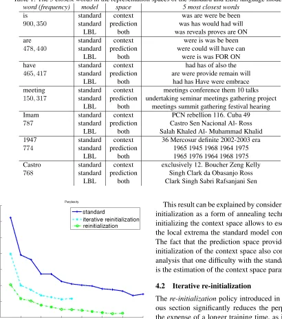
The evolution of the perplexity with respect to train-ing epochs for this new method is plotted on Fig-ure 2, where we only represent the evolution of the perplexity during the third training step. As can be seen, at convergence, the perplexity the model esti-mated with this technique is about 10% smaller than the perplexity of the standard model.

This result can be explained by considering the initialization as a form of annealing technique: re-initializing the context space allows to escape from the local extrema the standard model converges to. The fact that the prediction space provides a good initialization of the context space also confirms our analysis that one difficulty with the standard model is the estimation of the context space parameters.

4.2 Iterative re-initialization

There-initialization policy introduced in the previ-ous section significantly reduces the perplexity, at the expense of a longer training time, as it requires to successively train two models. As we now know that the parameters of the prediction space are faster to converge, we introduce a second training regime called iterative re-initializationwhich aims to take advantage of this property. We summarize this new training regime as follows:

1. Train the model for one epoch.

2. Use the prediction space parameters to reini-tialize the context space.

Figure 3: Evolution of the perplexity on the training data for various initialization regimes.

This regimes yields a model that is somewhat in-between the standard and LBL models as it adds a relationship between the two representation spaces, which lacks in the former model. This relationship is however not expressed through the tying of the cor-responding parameters; instead we let the prediction space guide the convergence of the context space. As a consequence, we hope that it can achieve a con-vergence speed as fast as the one of the LBL model without degrading its prediction capacity.

The result plotted on Figure 2 shows that this in-deed the case: using this training regime, we ob-tained a perplexity similar to the one of the stan-dard model, while at the same time reducing the total training time by more than a half, which is of great practical interest (each epoch lasts approxi-mately 8 hours on a 3GHz Xeon processor).

Figure 3 displays the perplexity convergence curve measured on the training data for the standard learning regime as well as for the re-initialization

and iterative re-initialization. These results show the same trend as for the perplexity measured on the development data, and suggest a regularization effect of the re-initialization schemes rather than al-lowing the models to escape local optima.

4.3 One vector initialization

Principle The new training regimes introduced above outperform the standard training regime both in terms of perplexity and of training time. However, exchanging information between the context and

prediction spaces is only possible when the same vocabulary is used in both spaces. As discussed in Section 2.4, this configuration is not realistic for very large-scale tasks. This is because increasing the number of predicted word types is much more com-putationally demanding than increasing the number of types in the context vocabulary. Thus, the former vocabulary is typically order of magnitudes larger than the latter, which means that the re-initialization strategies can no longer be directly used.

It is nonetheless possible to continue drawing in-spirations from the observations made in Section 3, and, crucially, to question the random initialization strategy. As discussed above, this strategy may ex-plain why the neighborhoods in the induced con-text space for the less frequent types were diffi-cult to interpret. As a straightforward alternative, we consider a different initialization strategy where all the words in the context vocabulary are initially projected onto the same (random) point in the con-text space. The intuition is that it will be easier to build meaningful neighborhoods, especially for rare types, if all words are initially considered similar and only diverge if there is sufficient evidence in the training data to suggest that they should. This model is termed theone vector initializationmodel.

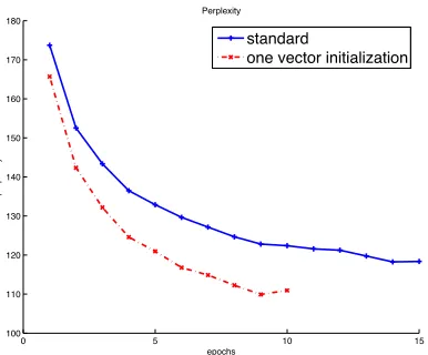
Experimental evaluation To validate this ap-proach, we compare the convergence of a standard model trained (with the standard learning regime) with the one vector initialization regime. The con-text vocabulary is defined by the532,557words oc-curring in the training data and the prediction vo-cabulary by the10,000most frequent words6. All other parameters are the same as in the previous experiments. Based on the curves displayed on Figure 4, we can observe that the model obtained with the one vector initialization regime outperforms the model trained with a completely random ini-tialization. Moreover, the latter reaches conver-gence in only 14 epochs, while the learning regime we propose only needs 9 epochs. Convergence is even faster than when we used the standard training regime and a small context vocabulary.

6

0 5 10 15 100

110 120 130 140 150 160 170 180

epochs

perplexity

Perplexity

standard

one vector initialization

Figure 4: Perplexity with all-10,000,200−200models

Table 2: Summary of the perplexity (PPX) results mea-sured on the same development set with the different con-tinuous space language models. For all of them, the prob-abilities are combined with the back-offn-gram model

Vcsize Model # epochs PPX 10000 log bilinear 6 239

standard 13 227

iterative reinit. 6 223

reinit. 11 211

all standard 14 276

one vector init. 9 260

To illustrate the impact of our initialization scheme, we also used a principal component anal-ysis to represent the induced word representations in a two dimensional space. Figure 5 represents the vectors associated with numbers7 in red, while all other words are represented in blue. Two different models are used: the standard model on the left, and the one vector initialization model on the right. We can observe that, for the standard model, most of the red points are scattered all over a large portion of the representation space. On the opposite, for the one vector initialization model, points associated with numbers are much more concentrated: this is simply because all the points are originally identi-cal, and the training aim to spread the point around this starting point. We also created the closest word list reported in Table 3, in a manner similar to Ta-ble 1. Clearly, the new method seems to yield more

7

Number are all the words consisting only of digits, with an optional sign, point or comma such as:1947;0,001;-8,2.

(a) with the standard model (b) with the one vector initial-ization model

Figure 5: Comparison of the word embedding in the con-text space for numbers (red points).

meaningful neighborhoods in the context space. It is finally noteworthy to mention that when used with a small context vocabulary (as in the experi-mental setting of Section 4.1) this initialization strat-egy underperforms the standard initialization. This is simply due to the much greater data sparsity in the large context vocabulary experiments, where the rarer word types are really rare (they typically occur once or twice). By contrast, the rarer words in the small vocabulary tasks occurred more than several hundreds times in the training corpus, which was more than sufficient to guide the model towards sat-isfactory projection matrices. This finally suggests that there still exists room for improvement if we can find more efficient initialization strategies than starting from one or several random points.

4.4 Statistical machine translation experiments

-Table 3: The 5 closest words in the context space of the standard and one vector initialization language models

word (freq.) model 5 closest words

is standard was are were been remains 900,350 1 vector init. was are be were been

conducted standard undertaken launched $270,900 Mufamadi 6.44-km-long 18,388 1 vector init. pursued conducts commissioned initiated executed Cambodian standard Shyorongi $3,192,700 Zairian depreciations teachers 2,381 1 vector init. Danish Latvian Estonian Belarussian Bangladeshi automatically standard MSSD Sarvodaya $676,603,059 Kissana 2,652,627 1,528 1 vector init. routinely occasionally invariably inadvertently seldom Tosevski standard $12.3 Action,3 Kassouma 3536 Applique 34 1 vector init. Shafei Garvalov Dostiev Bourloyannis-Vrailas Grandi October-12 standard 39,572 anti-Hutu $12,852,200 non-contracting Party’s 8 1 vector init. March-26 April-11 October-1 June-30 August4 3727th standard Raqu Tatsei Ayatallah Mesyats Langlois 1 1 vector init. 4160th 3651st 3487th 3378th 3558th

best list is accordingly reordered to produce the final translations.

The different language models discussed in this article are evaluated on the Arabic to English NIST 2009 constrained task. For the continuous space language model, the training data consists in the parallel corpus used to train the translation model (previously described in section 3.1). The de-velopment data is again the 2006 NIST test set and the test data is the official 2008 NIST test set. Our system is built using the open-source Moses toolkit (Koehn et al., 2007) with default settings. To set up our baseline results, we used an extensively op-timized standard back-off 4-grams language model using Kneser-Ney smoothing described in (Allauzen et al., 2009). The weights used during the reranking are tuned using the Minimum Error Rate Training algorithm (Och, 2003). Performance is measured based on the BLEU (Papineni et al., 2002) scores, which are reported in Table 4.

Table 4: BLEU scores on the NIST MT08 test set with different language models.

Vcsize Model # epochs BLEU

all baseline - 37.8

10000 log bilinear 6 38.2

standard 13 38.3

iterative reinit. 6 38.4

reinit. 11 38.4

all standard 14 38.6

one vector init. 9 38.7

All the experimented neural language models yield to a significant BLEU increase. The best re-sult is obtained by the one vector initialization stan-dard model which achieves a 0.9 BLEU improve-ment. While this results is similar to the one ob-tained with the standard model, the training time is reduced here by a third.

5 Conclusion

In this work, we proposed three new methods for training neural network language models and showed their efficiency both in terms of computa-tional complexity and generalization performance in a real-word machine translation task. These meth-ods rely on conclusions drawn from a careful study of the convergence rate of two state-of-the-art mod-els and are based on the idea of sharing the dis-tributed word representations during training.

Our work highlights the impact of the initializa-tion and the training scheme for neural network lan-guage models. Both our experimental results and our new training methods can be closely related to the pre-training techniques introduced by (Hinton and Salakhutdinov, 2006). Our future work will thus aim at studying the connections between our empir-ical observations and the deep learning framework.

Acknowledgments

References

Alexandre Allauzen, Josep Crego, Aur´elien Max, and Franc¸ois Yvon. 2009. LIMSI’s statistical transla-tion systems for WMT’09. In Proceedings of the Fourth Workshop on Statistical Machine Translation, pages 100–104, Athens, Greece, March. Association for Computational Linguistics.

Yoshua Bengio, R´ejean Ducharme, Pascal Vincent, and Christian Janvin. 2003. A neural probabilistic lan-guage model.JMLR, 3:1137–1155.

J. Bilmes, K. Asanovic, C. Chin, and J. Demmel. 1997. Using phipac to speed error back-propagation learn-ing. Acoustics, Speech, and Signal Processing, IEEE International Conference on, 5:4153.

Peter F. Brown, Peter V. deSouza, Robert L. Mercer, Vin-cent J. Della Pietra, and Jenifer C. Lai. 1992. Class-based n-gram models of natural language. Comput. Linguist., 18(4):467–479.

Stanley F. Chen and Joshua Goodman. 1996. An empiri-cal study of smoothing techniques for language model-ing. InProc. ACL’96, pages 310–318, San Francisco. Ronan Collobert and Jason Weston. 2008. A

uni-fied architecture for natural language processing: deep neural networks with multitask learning. In Proc.

of ICML’08, pages 160–167, New York, NY, USA.

ACM.

Ahmed Emami and Lidia Mangu. 2007. Empirical study of neural network language models for Arabic speech recognition. InProc. ASRU’07, pages 147–152, Ky-oto. IEEE.

Geoffrey E. Hinton and Ruslan R. Salakhutdinov. 2006. Reducing the dimensionality of data with neural net-works. Science, 313(5786):504–507, July.

Philipp Koehn, Hieu Hoang, Alexandra Birch, Chris Callison-Burch, Marcello Federico, Nicola Bertoldi, Brooke Cowan, Wade Shen, Christine Moran, Richard Zens, Chris Dyer, Ondrej Bojar, Alexandra Con-stantin, and Evan Herbst. 2007. Moses: Open source toolkit for statistical machine translation. In Proc. ACL’07, pages 177–180, Prague, Czech Republic. Philipp Koehn. 2010. Statistical Machine Translation.

Cambridge University Press.

Hong-Kwang Kuo, Lidia Mangu, Ahmad Emami, and Imed Zitouni. 2010. Morphological and syntactic fea-tures for arabic speech recognition. InProc. ICASSP 2010.

Raymond Lau, Ronald Rosenfeld, and Salim Roukos. 1993. Adaptive language modeling using the maxi-mum entropy principle. InProc HLT’93, pages 108– 113, Princeton, New Jersey.

Andriy Mnih and Geoffrey Hinton. 2007. Three new graphical models for statistical language modelling. In

Proc. ICML ’07, pages 641–648, New York, NY, USA.

Andriy Mnih and Geoffrey E Hinton. 2008. A scalable hierarchical distributed language model. In D. Koller, D. Schuurmans, Y. Bengio, and L. Bottou, editors, Ad-vances in Neural Information Processing Systems 21, volume 21, pages 1081–1088.

Thomas R. Niesler. 1997. Category-based statistical language models. Ph.D. thesis, University of Cam-bridge.

Franz Josef Och. 2003. Minimum error rate training in statistical machine translation. InProc. ACL’03, pages 160–167, Sapporo, Japan.

Ilya Oparin, Ondˇrej Glembek, Luk´aˇs Burget, and Jan ˇ

Cernock´y. 2008. Morphological random forests for language modeling of inflectional languages. InProc. SLT’08, pages 189–192.

Kishore Papineni, Salim Roukos, Todd Ward, and Wei-Jing Zhu. 2002. Bleu: a method for automatic evalu-ation of machine translevalu-ation. InProc. ACL’02, pages 311–318, Philadelphia.

Ronald Rosenfeld. 1996. A maximum entropy approach to adaptive statistical language modeling. Computer, Speech and Language, 10:187–228.

Holger Schwenk and Jean-Luc Gauvain. 2002. Connec-tionist language modeling for large vocabulary contin-uous speech recognition. InProc. ICASSP, pages 765– 768, Orlando, FL.

Holger Schwenk, Daniel D´echelotte, and Jean-Luc Gau-vain. 2006. Continuous space language models for statistical machine translation. In Proc. COL-ING/ACL’06, pages 723–730.

Holger Schwenk. 2007. Continuous space language models.Comput. Speech Lang., 21(3):492–518. Yeh W. Teh. 2006. A hierarchical Bayesian language

model based on Pitman-Yor processes. In Proc. of ACL’06, pages 985–992, Sidney, Australia.