Text Classification with Few Examples using Controlled Generalization

3158

Text Classification with Few Examples using Controlled Generalization

Abhijit Mahabal Google, Pinterest

amahabal@ gmail.com

Jason Baldridge Google

jridge@ google.com

Burcu Karagol Ayan Google

burcuka@ google.com

Vincent Perot Google

vperot@ google.com

Dan Roth UPenn

danroth@ seas.upenn.edu

Abstract

Training data for text classification is often limited in practice, especially for applications with many output classes or involving many related classification problems. This means classifiers must generalize from limited evi-dence, but the manner and extent of general-ization is task dependent. Current practice pri-marily relies on pre-trained word embeddings to map words unseen in training to similar seen ones. Unfortunately, this squishes many components of meaning into highly restricted capacity. Our alternative begins with sparse pre-trained representations derived from unla-beled parsed corpora; based on the available training data, we select features that offers the relevant generalizations. This produces task-specific semantic vectors; here, we show that a feed-forward network over these vectors is es-pecially effective in low-data scenarios, com-pared to existing state-of-the-art methods. By further pairing this network with a convolu-tional neural network, we keep this edge in low data scenarios and remain competitive when using full training sets.

1 Introduction

Modern neural networks are highly effective for text classification, with convolutional neural net-works (CNNs) as the de facto standard for clas-sifiers that represent both hierarchical and order-ing information implicitly in a deep network (Kim, 2014). Deep models pre-trained on language model objectives and fine-tuned to available train-ing data have recently smashed benchmark scores on a wide range of text classification problems (Peters et al.,2018;Howard and Ruder,2018; De-vlin et al.,2018).

Despite the strong performance of these ap-proaches for large text classification datasets, chal-lenges still arise with small datasets with few, pos-sibly imbalanced, training examples per class.

La-bels can be obtained cheaply from crowd workers for some languages, but there are a nearly unlim-ited number of bespoke, challenging text classifi-cation problems that crop up in practical settings (Yu et al.,2018). Obtaining representative labeled examples for classification problems with many labels, like taxonomies, is especially challenging.

Text classificationis a broad but useful term and covers classification based on topic, on sentiment, and even social status. As Systemic Functional Linguists such asHalliday (1985) point out, lan-guage carries many kinds of meanings. For exam-ple, words such asambrosialanddelishinform us not just of the domain of the text (food) and sen-timent, but perhaps also of the age of the speaker. Text classification problems differ on the dimen-sions they distinguish along and thus in the words that help in identifying the class.

AsSachan et al.(2018) show, classifiers mostly focus on sub-lexicons; they memorize patterns in-stead of extending more general knowledge about language to a particular task. When there is low lexical overlap between training and test data, ac-curacy drops as much as 23.7%. When training data is limited, most meaning-carrying terms are never seen in training, and the sub-lexicons cor-respondingly poorer. Classifiers must generalize from available training data, possibly exploiting external knowledge, including representations de-rived from raw texts. For small training sizes, this requires moving beyond sub-lexicons.

Existing strategies for low data scenarios in-clude treating labels as informative (Song and Roth,2014;Chang et al., 2008) and using label-specific lexicons (Eisenstein,2017), but neither is competitive when labeled data is plentiful. In-stead, we seek classifiers that adapt to both low and high data scenarios.

1.1 Kampuchea saysricecrop in 1986 increased. . . 2.1 Gamma rayBursters. What are they? 1.2 U.S.sugarpolicy may self-destruct. . . 2.2 Life onMars

1.3 EC deniesmaizeexports reserved for the U.S.. . . 2.3 Single launchspace stations

1.4 U.S.corn,sorghumpayments 50-50 cash/certs. . . 2.4 Astronauts—what does weighlessness feel like? 1.5 Canadacorndecision unjustified. . . 2.5 SatellitearoundPlutomission?

Table 1:Left: examples from the ReutersGrainsclass, showing semantic type cohesion (kinds of crops). Right: post headers from thesci.space newsgroup in 20 Newsgroups, showing topical cohesion (astronomical terms).

Bolded termsare to draw the reader’s attention to parallels among examples.

Sander, 2013). Consider Table 1, which displays five examples from a single class for two tasks. Bolded terms for each task are clearly related, and to a person, suggest abstractions that help relate other terms to the task. This helps with disam-biguation: that the wordPlutois the planet and not Disney’s character is inferred not just by within-example evidence (e.g.mission) but also by cross-example presence ofMarsandastronauts.

Cross-example analysis also reveals the amount of generalization warranted. For a word associated with a label, word embeddings give us neighbors, which often are associated with that label. What they do not tell us is the extent this associated-with-same-label phenomenon holds; that depends on the granularity of the classes. Cross-example analysis is required to determine how neighbors at various distances are distributed among labels in the training data. This should allow us to in-clude barley andpeaches as evidence for a class likeAgriculturebut onlybarleyforGrains.

Most existing systems ignore cross-example parallelism and thus miss out on a strong classi-fication signal. We introduce a flexible method for controlled generalization that selects syntacto-semantic features from sparse representations con-structed by Category Builder (Mahabal et al., 2018). Starting with sparse representations of words and their contexts, a tuning algorithm se-lects features with the relevant kinds and appro-priate amounts of generalization, making use of parallelism among examples. This produces task-specific dense embeddings for new texts that can be easily incorporated into classifiers.

Our simplest model, CBC (Category Builder Classifier), is a feed-forward network that uses only CB embeddings to represent a document. For small amounts of training data, this simple model dramatically outperforms both CNNs and BERT (Devlin et al.,2018). When more data is available, both CNNs and BERT exploit their greater capac-ity and broad pre-training to beat CBC. We thus create CBCNN, a simple combination of CBC and

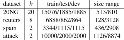
dataset k train/test/dev size range 20NG 20 15076/1885/1885 513/810 reuters 8 6888/862/864 128/3128 spam 2 3344/1115/1115 436/2908 attack 2 10000/2000/2000 1126/8874

Table 2: Data sizes, and the disparity between the smallest and the largest class in training data. Thek

column indicates the number of classes in the task.

the CNN that concatenates their pre-prediction layers and adds an additional layer. By training this model with a scheduled block dropout (Zhang et al., 2018) that gradually introduces the CBC sub-network, we obtain the benefits of CBC in low data scenarios while obtaining parity with CNNs when plentiful data is available. BERT still dom-inates when all data is available, suggesting that further combinations or ensembles are likely to improve matters further.

2 Evaluation Strategy

Our primary goal is to study classifier performance with limited data. To that end, we obtain learning curves on four standard text classification datasets (Table 2) based on evaluating predictions on the full test sets. At each sample size, we produce multiple samples and run several text classification methods multiple times, measuring the following:

• Macro-F1 score. Macro-F1 measures sup-port for all classes better than accuracy, espe-cially with imbalanced class distributions.

• Recall for the rarest class. Many measures like F1 and accuracy often mask performance on infrequent but high impact classes, such as detecting toxicity (Waseem and Hovy,2016))

The datasets we chose for evaluation, while all multi-class, form a diverse set in terms of the num-ber of classes and kinds of cohesion among exam-ples in a single class. The former clearly affects training data needs, while the latter informs ap-propriate generalization.

• 20 Newsgroups20Newsgroups (20NG) con-tains documents from 20 different news-groups with about 1000 messages from each. We randomly split the documents into an 80-10-10 train-dev-test split. The classes are evenly balanced.

• Reuters R8. The Reuters21578 dataset con-tains Reuters Newswire articles. Following several authors (Pinto and Rosso,2007;Zhao et al., 2018, for example), we use only the eight most frequent labels. We begin with a given 80/10/10 split. Given that we fo-cused on single-label classification, we re-moved items associated with two or more of the top eight labels (about 3% of exam-ples). Classes are highly imbalanced. Of the 6888 training examples, 3128 are labeled earn, while only 228 examples are of class interestand only 128 areship.

• Wiki Comments Personal Attack. The Wikipedia Detox project collected over 100k discussion comments from English Wikipedia and annotated them for presence of personal attack (Wulczyn et al.,2017). We randomly select 10k, 2k, and 2k items as train/dev/test. 11% are attacks.

• Spam The SMS Spam Collection v.1 has SMS labeled messages that were collected for mobile phone spam research (Hidalgo et al., 2012). Each of the 5574 messages is labeled asspamorham.

3 Identifying Generalizing Features

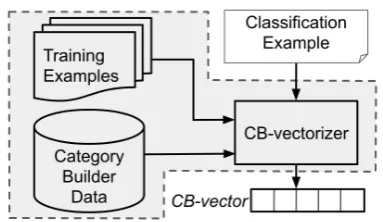
In this section, we explicate the source of fea-tures, discuss the properties relevant to generaliza-tion by focusing on one feature in isolageneraliza-tion, and present the overall feature selection method. The overview in Figure 1displays the order of opera-tions: identify generalizing featuresbased on the training data (done once), and for each document to be classified, convert it to a vector, where each entry corresponds to a generalizing feature.

Figure 1: Shaded Region: We use Category Builder data (Mahabal et al., 2018) and identify generalizing features in training data, producing avectorizer. This is done once. Unshaded:Given a document, the vector-izer produces a dense vector usable in deep networks.

Feature Prototypical Supports

allergen as X pollen, dander, dust mites, soy, perfumes, milk, smoke, mildew liter of X water, petrol, milk, fluid, beer serve with X rice, sauce, salad, fries, milk flour mixture butter mixture, rubber

spat-ula, dredged, creamed, medium speed, sifted, milk

replacer colostrum, calves, whole milk, inulin, pasteurized, weaning

Table 3: A few features (among hundreds) evoked by

milk, with top n-grams in their support.Above dashed line (FS)fit in tidy categories (here,allergen,fluid, and foodare rough glosses). Below dashed line (FC)are

not describable by simple labels—the evoking terms have different parts of speech and instead display

sit-uational coherence, e.g. association with the process

of mixing flour or with animal husbandry (areplaceris milk formula for calves).

3.1 Category Builder

pointwise-mutual information (Mahabal et al.,2018).

3.2 Properties of Generalizing Features

Which features generalize well depends on the granularity of classes in a task. Useful features for generalization strike a balance between breadth andspecificity. A feature that is evoked by many words provides generalization potential because the feature’s overall support is likely to be dis-tributed across both the training data and test data. However, this risks over-generalization, so a fea-ture should also be sufficiently specific to be a pre-cise indicator of a particular class.

A key aspect of choosing good features based on a limited training set is to resolve referential ambiguity (Quine, 1960; Wittgenstein, 1953) to the extent supported by the observed uses of the words. To illustrate, consider the grainsclass in the Reuters Newswire dataset. The word wheat can evoke the features at different levels of the taxonimical hierarchy:triticum(the wheat genus), poaceae (grass family), spermatophyta (seeded plants),plantae(plant kingdom), andliving thing. The first among these has low breadth and is evoked only bywheat. The second is far more use-ful: specific and yet with a large support, including maizeandsorghum. The final feature is too broad. In general, the most useful features for generaliza-tion are the intermediate features, also known as Basic Level Categories (Rosch et al.,1976).

Another important aspect of generalization comprises the facets of meaning. For example, the wordmilkhas facets relating it to other liquids (e.g., oil, kerosene), foods (cheese, pasta), white things (ivory), animal products (honey,eggs), and allergens (pollen, ragweed). Along these axes, generalization can be more or less conservative; e.g., bothcheeseandtears of a phoenixare animal products, but the former is semantically closer to milk. Looking back at Table3, the utility of indi-vidual features evoked bymilkfor tasks involving related topics varies; e.g., does the classification problem pertain tofoodoranimal husbandary?

3.3 Focus on a single feature

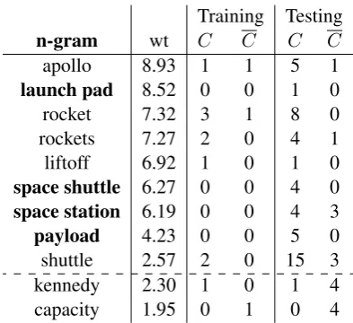
A single generalizing feature is associated with many n-grams, each of which evokes it (with dif-ferent strengths). Table 4 displays n-grams that evoke the featureco-occurrence withSaturn V, as discovered by unsupervised analysis of a large cor-pus of web pages. The table further displays the interaction of this unsupervised feature with

super-Training Testing

n-gram wt C C C C

apollo 8.93 1 1 5 1

launch pad 8.52 0 0 1 0

rocket 7.32 3 1 8 0 rockets 7.27 2 0 4 1 liftoff 6.92 1 0 1 0

space shuttle 6.27 0 0 4 0

space station 6.19 0 0 4 3

payload 4.23 0 0 5 0

shuttle 2.57 2 0 15 3 kennedy 2.30 1 0 1 4 capacity 1.95 0 1 0 4

Table 4: Some evoking n-grams associated with the CB featureco-occurrence withSaturn Vand pivoting on the class sci.space. Counts for n-grams in train-ing (sample size 320) and test data are shown, within

sci.space (C) and outside (C). Bolded n-grams are

not seen in training but occur in test, providing gen-eralization. The dashed line represents a threshold; higher scoring n-grams are more cohesive, and thresh-olding can make a feature cleaner by decreasing seman-tic drift.

vised data, specifically, with the labelsci.spacein 20NG, when using a size 320 training sample that contain only 18sci.spacedocuments. Counts for some evoking terms are shown within and outside this class, for both training and test data.

Notation. We introduce some notation and ex-plicate with Table 4. We have a labelled collec-tion of training documents T. Tl is the training examples with label l. The positive support set

Ψl(f, t)is the set of n-grams inTlevoking feature

fwith weight greater thant, here,{apollo, rocket, . . . , shuttle}fort=2.3. The positive support size

Λl(f,2.3)=|Ψl(f,2.3)|=5 and the positive

sup-port weightλl(f,2.3)is the sum of counts of sup-ports off inlwith weight greater than 2.3, here

1+3+2+1+2=9. Analogously thenegative

sup-port weight λ_l(f,2.3)is the sum of counts from outside Tl; here, 1+1=2 since {apollo, rocket} were seen outsidesci.spaceonce each.

exam-ple; our methods do not access the test data for feature selection in our experiments.)

That said, we must limit potential noise from such features, so we seek thresholded features

hf, ti, as suggested by the dashed line in Table 4. Items below this line are prevented from evok-ingf. We choose the highest threshold such that dropped negative support exceeds dropped posi-tive support. This is determined simply by go-ing through all the supports of a feature, sorted by ascending weight, and checking the positive and negative support of all features with smaller ver-sus greater weight given the class. The weight of the feature at this cusp is used as the threshold of the feature for this particular class. Thishf, tipair then forms one element of the CB-vector used as a feature for classification.

Given the labeled subsets ofT and this feature thresholding algorithm, we produce a vectorizer that embeds documents. The values of a docu-ment’s embeddingare notdirectly associated with any class. Such association happens during train-ing. Although sci.space accounts for just 6% of the documents, 75% of documents that contain an n-gram evoking the Saturn V feature are in that class. A classifier trained with such an embed-ding should learn to associate this feature with that class, and an unseen document containing the unseen-in-training termspace shuttlestands a good chance to be classified assci.space.

The feature displayed in Table4is useful for the 20NG problem because it contains a class related to space travel. This feature has no utility in spam classification or in sentiment classification, since, for those problems, seeingrocketin one class does not make it more likely that a document contain-ingspace stationbelongs to that same class. This example illustrates why a generalization strategy must incorporate both what we can learn from un-supervised data as well as (limited) labeled train-ing data.

3.4 Overall feature selection

We now describe how we use the training dataT

to produce a set of features-and-threshold pairs; each chosen feature-with-threshold hf, ti will be one component in the CB-vectors provide to clas-sifiers. Calculation of features for a single class is a three step process: (i) for each featuref, choose a thresholdt(as discussed above) (ii) score the re-sultanthf, ti(iii) filter useless or redundanthf, ti.

Given a label l and a feature f, we implicitly produce a table of supporting n-grams and their distribution within and outsidel(e.g. as in Table 4). This involves computing the precision of a fea-ture at a given threshold value, comparing it to the class probability and deciding whether to keep it.

Recall the positive supportλl(f, t)and negative support λ_f(f, t) defined previously. The preci-sionoffat thresholdtisµl(f, t) = _λl(f,tλl(₎₊f,t_λ)

l(f,t),

(this is ₁₁9 in the example of Table4, witht=2.3). However, since we are often dealing with low counts, we smooth the precision toward the em-pirical class probability ofl,p(l) = |Tl|

|Tl|+|Tl|.

˜

µl(f, t) =

λl(f, t) +p(l)α

λl(f, t) +λl(f, t) +α

The score Sl(f, t) is reduction in error rate of the smoothed precision relative to the base rate:

Sl(f, t) =

˜

µl(f, t)−p(l)

1−p(l)

We retain a thresholded feature if it is generalizing (Λl(hf, ti)> 1), has better-than-chance precision (we useSl(hf, ti) > 0.01), and is not redundant (i.e., its positive support has one or more terms not present in positive supports of higher scoring fea-tures).

3.5 Creating the CB-vector

Each vector dimension corresponds to somehf, ti. The evocation level of f is the sum of its evoca-tion for the n-grams in the documentd,ed(f) = P

w∈dCB(w, f). The vector entry is ed(f)

t when

ed(f)>=t, and is clipped to0otherwise.

4 Models

As benchmarks, we use a standard CNN with pre-trained embeddings (Kim,2014) and BERT ( De-vlin et al., 2018).1 For CNN, we used 300 filters each of sizes 2, 3, 4, 5, and 6, fed to a hidden layer of 200 nodes after max pooling. Pretrained vectors provided by Google were used.2 For BERT, we used the run classifierscript from GitHub and used the BERT-large-uncased model.

We use the pre-computed vocab-to-context as-sociation matrix provided as part of the open

1

https://github.com/google-research/bert

2

source Categorial Builder repository.3 This con-tains 194,051 co-occurrence features (FC) and 954,276 syntactic features (FS).

CBC model. TheCB-vectorcontaining the de-rived features from the training dataset and Cate-gory Builder can be exploited in various ways with existing techniques. The simplest of these is to use a feed-forward network over theCB-vector. This model does not encode the tokens or any word or-der information—information which is highly in-formative in many classification tasks.

CBCNN model. Inspired by the combination of standard features and deep networks in Wide-and-Deep models (Cheng et al.,2016), we pair the CBC model with a standard CNN, concatenating their pre-prediction layers, and add an additional layer before the softmax prediction. In early ex-periments, this combined model performed worse than the CNN on larger data sizes, as the network above the CB-vector effectively stole useful signal from the CNN. To ensure that the more complex CNN side of the network had a chance to train, we employed a block dropout strategy (Zhang et al., 2018) with a schedule. During training, with some probability, all weights in the CB-vector are set to 0.5. The probability of hiding decreases from 1 to 0 using a parameterized hyperbolic tangent func-tionpk=_eCx2₊₁. Lower values ofClead to slower

convergence to zero. The effect is that the CBC sub-network is introduced gradually, allowing the CNN to train while eventually taking advantage of the additional information.

The natural strategy of replacing with 0s (in-stead of 0.5 as above) was tried and also works, but less well, since the network has no way to dis-tinguish between genuine absence of feature and hiding. In CB-vector, non-zero values are at least 1, and thus 0.5 does not suffer from this problem.

5 Experiments

Our primary goal is to improve generalization for low-data scenarios, but we also want our methods to remain competitive on full data.

5.1 Experimental setup

We compare different models across learning curves of increasing the training set sizes. We use training data sizes of 40,80, . . . ,5120 as well as the entire available training data. For each train-ing size, we produce three independent samples

3

https://github.com/google/categorybuilder

by uniformly sampling the training data and train-ing each model three times at each size. The fi-nal value reported is the average of all nine runs. All models are implemented in Tensorflow. Batch sizes are between 5 and 64 depending on training size. Training stops after there is no macro-F1 im-provement on development data for 1000 steps.

For evaluation, we focus primarily on macro-F1 and recall of the rarest class. The recall on the rarest class is especially important for imbal-anced classification problems. For such problems, a model can obtain high accuracy by strongly pre-ferring the majority class, but we seek models that effectively identify minority class labels. (This is especially important for active learning scenarios, where we expect the CB-vectors to help with in future.)

5.2 Results: low data scenarios

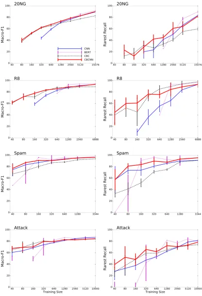
Figure2 shows learning curves giving macro-F1 scores and rarest class recall for all four datasets. When very limited training data is available, the simple CBC model generally outperforms the CNN and BERT, except for the Spam dataset. The more powerful models eventually surpass CBC; however, the CBCNN model provides consistent strong performance at all dataset sizes by combin-ing the generalization of CBC with the general ef-ficacy of CNNs. Importantly, CBCNN provides massive error reductions with low data for 20NG and R8 (tasks with many labels).

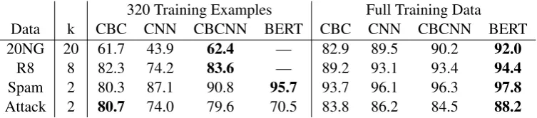
Table 5’s left half gives results for all mod-els when using only 320 training examples. For 20NG, CNN’s macro-F1 is just 43.9, whereas CBC and CBCNN achieve 61.7 and 62.4—the same as CNN performance with four times as much data. These models outperform CNN on R8 as well, reaching 83.7 vs CNN’s 74.1, and also on the Wiki-attack dataset, achieving 80.6 vs CNNs 74.0. BERT fails to produce a solution for the two datasets with>2 labels, but does produce the best result for Spam—indicating an opportunity to more fully explore BERT’s parameter settings for low data scenarios and to fruitfully combine CBC with BERT.

inter-40 80 160 320 640 1280 2560 5120 15076 0

20 40 60 80 100

Ma

cro

-F1

20NG

CNN BERT CBC CBCNN

40 80 160 320 640 1280 2560 5120 15076

0 20 40 60 80 100

Ra

rest

Re

ca

ll

20NG

40 80 160 320 640 1280 2560 6888

0 20 40 60 80 100

Ma

cro

-F1

R8

40 80 160 320 640 1280 2560 6888

0 20 40 60 80 100

Ra

rest

Re

ca

ll

R8

40 80 160 320 640 1280 3344

0 20 40 60 80 100

Ma

cro

-F1

Spam

40 80 160 320 640 1280 3344

0 20 40 60 80 100

Ra

rest

Re

ca

ll

Spam

40 80 160 320 640 1280 2560 5120 10000

Training Size

0 20 40 60 80 100

Ma

cro

-F1

Attack

40 80 160 320 640 1280 2560 5120 10000

Training Size

0 20 40 60 80 100

Ra

rest

Re

ca

ll

Attack

320 Training Examples Full Training Data Data k CBC CNN CBCNN BERT CBC CNN CBCNN BERT 20NG 20 61.7 43.9 62.4 — 82.9 89.5 90.2 92.0

R8 8 82.3 74.2 83.6 — 89.2 93.1 93.4 94.4

Spam 2 80.3 87.1 90.8 95.7 93.7 96.1 96.3 97.8

Attack 2 80.7 74.0 79.6 70.5 83.8 86.2 84.5 88.2

Table 5: Macro-F1 scores on all data sets when using 320 training examples (left) and when using all available training data (right). kis the number of classes. The CBCNN model provides the strongest overall performance across all data sizes. (Note that BERT produces degenerate solutions for the>2 class problems with 320 examples.)

Model k CBC CNN CBCNN BERT

20NG 20 80 320 80 1280

R8 8 40 160 40 640

Spam 2 40 40 40 40

Attack 2 40 40 40 40

Table 6: Minimum training size at which a non-degenerate model was produced in any of 9 runs. With more classes, more data is needed by CNN and BERT to produce acceptable models. k is number of classes.

acts with other strategies for dealing with limited resources, such as active learning. For example, Baldridge and Osborne (2008) obtained stronger data utilization ratios with better base models and uncertainty sampling for Reuters text classifica-tion: better models pick better examples for an-notation and thus require fewer new labeled data points to achieve a given level of performance.

Importantly, the CBC and CBCNN models take far less data to produce non-degenerate models (defined as a model which produces all output classes as predictions). CNN and BERT have a large number of parameters, and using these pow-erful tools with small training sets produces un-stable results. Table6gives the minimum training set sizes at which each model produces at least one non-degenerate model. While it might be possible to ameliorate the instability of CNN and BERT with a wider parameter search and other strate-gies, nothing special needs to be done for CBC. It is likely that an approach which adaptively se-lects CBC or CBCNN and BERT would obtain the strongest result across all training set sizes.

For each dataset, among the 100 best features chosen (for training size 640), the breakdown of domain features (FC) versus type features (FS) is revealing. As expected, domain features are more important in a topical task such as 20NG (71% are FC features), while the opposite is true for Spam (19%) and a toxicity dataset like Wiki

At-tack (23%). Reuters shows a fairly even balance between the two types of features (41%): it is use-ful for R8 to be topically coherent and also to hone in on fairly narrow groups of words that collec-tively cover a Basic Level Category.

5.3 Results: full data scenarios

Table 5provides macro-F1 scores for all models when given all available training data. The CBC model performs well, but its (intentional) igno-rance of the actual tokens in a document takes a toll when more labeled documents are avail-able. The CNN benchmark, which exploits both word order and the tokens themselves, is a strong performer. The CBCNN model effectively keeps pace with the CNN—improving on 20NG and R8, though slipping on Wiki-Attack. BERT sim-ply crushes all other models when there is suffi-cient training data, showing the impact of struc-tured pre-training and consistent with performance across a wide range of tasks inDevlin et al.(2018).

6 Conclusion

sources’ strengths—for example,FC features are like topics, andFS features like nodes in ontolo-gies. Nonetheless, a combination may add value.

Our focus is on data scarce scenarios. However, it would be ideal to derive utility at both the small and large labeled data sizes. This will likely re-quire models that can generalize with contextual features while also exploiting implicit hierarchical organization and order of the texts, e.g. as done by CNNs and BERT. The CBCNN model is one ef-fective way to do this and we expect there could be similar benefits from combining CBC with BERT. Furthermore, approaches like AutoML (Zoph and Le, 2017) would likely be effective for exploring the design space of network architectures for rep-resenting and exploiting the information inherent in both signals.

Finally, although we focus on multi-class prob-lems here—each example belongs to a single class—the general approach of selecting features should work for multi-label problems. Our confi-dence in this (unevaluated) claim stems from the observation that we select features one class at a time, treating that class and its complement as a binary classification problem.

Acknowledgements

We would like to thank our anonymous review-ers and the Google AI Language team, especially Rahul Gupta, Tania Bedrax-Weiss and Emily Pitler, for the insightful comments that contributed to this paper.

References

Jason Baldridge and Miles Osborne. 2008. Active learning and logarithmic opinion pools for HPSG parse selection. Natural Language Engineering, 14(2):191222.

David M. Blei, Andrew Ng, and Michael Jordan. 2003. Latent Dirichlet Allocation.JMLR, 3:993–1022.

Stephan Bloehdorn and Andreas Hotho. 2004. Boost-ing for text classification with semantic features. In

International Workshop on Knowledge Discovery on

the Web, pages 149–166. Springer.

Ming-Wei Chang, Lev Ratinov, Dan Roth, and Vivek Srikumar. 2008.Importance of semantic representa-tion: Dataless classification. InAAAI.

Heng-Tze Cheng, Levent Koc, Jeremiah Harmsen, Tal Shaked, Tushar Chandra, Hrishi Aradhye, Glen An-derson, Greg Corrado, Wei Chai, Mustafa Ispir, Ro-han Anil, Zakaria Haque, LicRo-han Hong, ViRo-han Jain,

Xiaobing Liu, and Hemal Shah. 2016. Wide & deep learning for recommender systems. In Proceed-ings of the 1st Workshop on Deep Learning for

Rec-ommender Systems, DLRS 2016, pages 7–10, New

York, NY, USA. ACM.

Jacob Devlin, Ming-Wei Chang, Kenton Lee, and Kristina Toutanova. 2018. BERT: Pre-training of deep bidirectional transformers for language under-standing. arXiv preprint arXiv:1810.04805.

Jacob Eisenstein. 2017. Unsupervised learning for lexicon-based classification. In Proceedings of the National Conference on Artificial Intelligence

(AAAI).

Katrin Erk. 2012. Vector space models of word mean-ing and phrase meanmean-ing: A survey. Language and

Linguistics Compass, 6(10):635–653.

Evgeniy Gabrilovich and Shaul Markovitch. 2009. Wikipedia-based semantic interpretation for natural language processing. Journal of Artificial

Intelli-gence Research, 34:443–498.

M. A. K. Halliday. 1985.An introduction to functional

grammar. Arnold.

Jose Maria Gomez Hidalgo, Tiago A Almeida, and Akebo Yamakami. 2012. On the validity of a new SMS spam collection. InProceedings of the 11st

ICMLA, volume 2, pages 240–245. IEEE.

Douglas Hofstadter and Emmanuel Sander. 2013. Sur-faces and essences: Analogy as the fuel and fire of

thinking. Basic Books.

Douglas R Hofstadter. 2001. Analogy as the core of cognition. The Analogical Mind: Perspectives from

Cognitive Science, pages 499–538.

Jeremy Howard and Sebastian Ruder. 2018. Univer-sal language model fine-tuning for text

classifica-tion. InProceedings of the 56th Annual Meeting of

the Association for Computational Linguistics

(Vol-ume 1: Long Papers), pages 328–339, Melbourne,

Australia.

Yoon Kim. 2014. Convolutional neural networks for sentence classification. In Proceedings of the 2014 Conference on Empirical Methods in Natural

Language Processing (EMNLP), pages 1746–1751,

Doha, Qatar.

Abhijit Mahabal, Dan Roth, and Sid Mittal. 2018. Ro-bust handling of polysemy via sparse representa-tions. In Proceedings of the Seventh Joint

Con-ference on Lexical and Computational Semantics,

pages 265–275.

Matthew Peters, Mark Neumann, Mohit Iyyer, Matt Gardner, Christopher Clark, Kenton Lee, and Luke Zettlemoyer. 2018. Deep contextualized word rep-resentations. In Proceedings of the 2018 Confer-ence of the North American Chapter of the Associ-ation for ComputAssoci-ational Linguistics: Human

Lan-guage Technologies, Volume 1 (Long Papers), pages

David Pinto and Paolo Rosso. 2007. On the rela-tive hardness of clustering corpora. InInternational

Conference on Text, Speech and Dialogue, pages

155–161. Springer.

Willard Van Orman Quine. 1960. Word and object. MIT press.

Eleanor Rosch, Carolyn B Mervis, Wayne D Gray, David M Johnson, and Penny Boyes-Braem. 1976. Basic objects in natural categories. Cognitive

psy-chology, 8(3):382–439.

Devendra Sachan, Manzil Zaheer, and Ruslan Salakhutdinov. 2018. Investigating the working of text classifiers. InProceedings of the 27th

Interna-tional Conference on ComputaInterna-tional Linguistics,

pages 2120–2131, Santa Fe, New Mexico, USA.

Yangqiu Song and Dan Roth. 2014. On dataless hier-archical text classification. InAAAI.

Zeerak Waseem and Dirk Hovy. 2016. Hateful sym-bols or hateful people? predictive features for hate speech detection on twitter. In Proceedings of the

NAACL Student Research Workshop, pages 88–93,

San Diego, California.

Ludwig Wittgenstein. 1953. Philosophical

investiga-tions. John Wiley & Sons.

Ellery Wulczyn, Nithum Thain, and Lucas Dixon. 2017. Ex machina: Personal attacks seen at scale.

InProceedings of the 26th International Conference

on World Wide Web, pages 1391–1399. International

World Wide Web Conferences Steering Committee.

Mo Yu, Xiaoxiao Guo, Jinfeng Yi, Shiyu Chang, Saloni Potdar, Yu Cheng, Gerald Tesauro, Haoyu Wang, and Bowen Zhou. 2018. Diverse few-shot text clas-sification with multiple metrics. In Proceedings of the 2018 Conference of the North American Chap-ter of the Association for Computational Linguistics: Human Language Technologies, Volume 1 (Long

Pa-pers), pages 1206–1215, New Orleans, Louisiana.

Yuan Zhang, Jason Riesa, Daniel Gillick, Anton Bakalov, Jason Baldridge, and David Weiss. 2018.

A fast, compact, accurate model for language identi-fication of codemixed text. In Proceedings of the 2018 Conference on Empirical Methods in

Natu-ral Language Processing, pages 328–337, Brussels,

Belgium.

Taotao Zhao, Xiangfeng Luo, Wei Qin, Subin Huang, and Shaorong Xie. 2018. Topic detection model in a single-domain corpus inspired by the human mem-ory cognitive process. Concurrency and

Computa-tion: Practice and Experience, 30(19):e4642.

Barret Zoph and Quoc V Le. 2017. Neural architecture search with reinforcement learning. InProceedings of the International Conference on Learning

Repre-sentations (ICLR).

A Appendix

Changes to the Category Builder Matrix

Category Builder uses two matrices: one mapping items to features (MV→F), the other mapping fea-tures to items (MF →V). Two are needed since the relationship is asymmetric: the featureX is a star signis more strongly associated with the term can-certhan vice versa, and the two matrices are thus not exact transposes of each other, although they almost are. For this current work, we just use one matrix,MV→F. For syntactic featuresFS, we di-rectly use the Category Builder rows. ForFC fea-tures, however, Category Builder replaced the cor-responding submatrix in MV→F with an identity matrix as described in (Mahabal et al.,2018). We obtain that part of the matrix by copying the cor-responding rows from(MF →V)T_.