A Proposal of a Smart Access Point Allocation Algorithm for Scalable Wireless Mesh Networks

(1)

A Proposal of a Smart Access Point Allocation

Algorithm for Scalable Wireless Mesh Networks

Kanako Uemura, Nobuo Funabiki, Toru Nakanishi

∗

Abstract—As a ﬂexible, inexpensive, and exten-sive Internet access network, we have studied

WIM-NET (Wireless Internet-access Mesh WIM-NETwork)

com-posed of multiple access points (APs) as wireless mesh routers. WIMNET utilizes two types of APs to achieve the scalability with suﬃcient bandwidth while reducing costs. One is the expensive, programmable

smart AP (SAP)that can use plural channels for wire-less communications and has various functions for the Internet access. Another is the inexpensive, non-programmable conventional AP (CAP) that can use only one channel. To enhance the performance, the proper SAP allocation is critical, because the num-ber of SAPs is much smaller than that of CAPs. In this paper, we present the definition of the SAP al-location problem, and its algorithm of extracting the optimum solution in terms of the newly defined cost function after finding the communication route con-figuration by applying our previous algorithms. We verify the effectiveness through simulations in three network topologies using the WIMNET simulator.

Keywords: Wireless mesh network, smart access point, allocation, algorithm, communication route

1 Introduction

Recently, IEEE.802.11 wireless local area networks

(WLANs) have been extensively used as ubiquitous In-ternet access networks. The WLAN does not require the wired cable connecting a host with an access point (AP) that is a connection hub with a wired network. Thus, the WLAN has several advantages such as the low network installation cost, the easy host relocation, and the ﬂexible communication area. As a result, the WLAN has been installed in a variety of places and institutions including governments, companies, homes, and schools. The public WLAN service has become popular in airports, stations, hotels, and even streets.

In the IEEE.802.11 WLAN, each AP can cover the

lim-ited area within approximately 100mdistance from it due

to the weak transmission signal. Thus, a single AP can-not oﬀer the network service to the broad area, where multiple APs are necessary for the service.

Convention-∗_{Dept. of Communication Network Engineering, Okayama}

Uni-versity, 3-1-1 Tsushimanaka, Okayama, 700-8530, Japan Email: [email protected]

ally, these APs are connected through wired cables. How-ever, the cabling cost may impair the cost advantage of the WLAN, and even the cable may not be able to be laid down in places such as outdoors and old buildings. As a way to solve this problem, the APs are allocated in mesh, and the adjacent APs are communicated with wireless links in addition to wireless communications be-tween APs and hosts. Communications bebe-tween distance APs are realized by the multihop fashion, where their in-termediate APs act as repeaters to reply packets. This

multihop WLAN is called thewireless mesh network[1].

Currently, a variety of styles have been studied for the wireless mesh network. Among them, this paper adopts the one that uses only APs as wireless mesh routers and

connects APs mainly on the MAC layer using the

wire-less distribution system (WDS). At least one AP acts as agateway (GW)to the Internet, where any host can con-nect to the Internet through a GW. For convenience, this

wireless mesh network has been calledWIMNET

(Wire-less Internet-access Mesh NETwork)in our studies [2].

When the size of WIMNET is expanded with the increas-ing number of APs and hosts, it may meet two serious

problems. One problem is the increase of

communica-tion delaydue to the bandwidth shortage at the wireless links around the GW, because increasing traﬃcs between the Internet and WIMNET must pass through the GW, whereas the bandwidth of those links is limited. Another

problem is thedegradation of dependability and

communi-cation qualitydue to the increasing interference between wireless links. As a result, the number of APs has been limited for WDS to avoid the unacceptable interference.

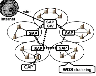
In order to solve these problems, we have proposed the hierarchical structure for the large-size WIMNET, which

is composed of the GW clusters and the WDS cluster.

As shown in Fig. 1, one GW cluster consists of the APs sharing the same GW, and one WDS cluster con-sists of the APs exchanging the same routing informa-tion for WDS. Besides, we have proposed the use of two

types of APs, namely the expensive, programmablesmart

(2)

one channel. Then, one WDS cluster consists of one SAP

as the cluster head and multiple CAPs where its

num-ber is limited, and one GW cluster consists of multiple WDS clusters. The WDS clusters are connected through SAPs with plural channels because their traﬃcs are usu-ally larger than those inside the WDS cluster. Then, the proper SAP allocation among APs becomes very impor-tant because it determines the performance and the cost of WIMNET.

SAP SAP

Internet

WDS clustering

CAP

SAP GW

wire

SAP

SAP SAPSAP SAP SAP SAP

SAP Internet

WDS clustering

CAP

SAP GW

[image:2.595.87.254.194.326.2]

wire

Figure 1: A GW cluster in WIMNET

In this paper, we define the SAP allocation problem for WIMNET, and present its algorithm. To maximize the performance of WIMNET, the minimization of the max-imum transmission time or delay per channel is signifi-cant. The transmission time can be obtained by the traf-fics among the interfered links using the same channel. Because the interfered links can be obtained only after the routing and NIC/channel assignments are fixed, the proposed algorithm applies our previous routing tree and NIC/channel assignment algorithms in [4] for any feasible SAP allocation satisfying the constraints of the problem.

Besides, themaximum estimated SAP loadis adopted to

prune undesirable SAP allocations oﬀering unbalanced SAP loads [5] to reduce the computation time.

To evaluate our proposal, we simulate the throughput of the SAP allocation found by our algorithm, using the WIMNET simulator. As simulated network topologies, we adopt two artificial ones with small numbers of SAPs where APs are located on grids and the center AP is se-lected as the GW, and another practical one that models the JR Okayama station [6]. In addition, two different traffic patterns are prepared to each grid topology. Any simulation result indicates that the SAP allocation by our algorithm gives the maximum throughput that is similar to the all-SAP case. We conclude that using our pro-posal, a large scale WIMNET can be made up with a small number of expensive high-performance SAPs.

The rest of this paper is organized as follows: Section 2 deﬁnes the SAP allocation problem. Section 3 presents the algorithm. Section 4 shows evaluation results by sim-ulations. Section 5 concludes the paper with some future

works.

2 Definition of SAP Allocation

Problem

For the inputs to the SAP allocation problem, we assume that the AP network topology, the GW, the maximum ex-pected number of associated hosts with each AP as loads, the interference among links, the transmission speed for each link, the WDS cluster size limit, and the channel interference matrix are given. As the output, the SAP allocation with the routing tree and NIC/channel assign-ments is requested to minimize the maximum

transmis-sion time. Then, the SAP allocation problem can be

formulated as follows:

A. Input:

• the AP network topology: G= (V, E)

– the number of APs: N =|V|

– the links between APs: E

– the interference among links: D = [dijpq],

where dijpq = 1 if two links, APi → APj and

APp →APq, are interfered, and dijpq = 0

oth-erwise

– the bandwidth oflinkij: sij (Mbps)

– the maximum expected number of associated

hosts withAPi: hi

– the Internet gateway: g (∈V)

• the number of SAPs: M

• the WDS cluster size (the maximum number of

CAPs in one WDS cluster): W SIZE

• the channel interference matrix: C= [c(i, j)]

• the number of channels: P

• the maximum number of NICs per SAP:Q

B. Output: the SAP allocation with the routing tree and NIC/channel assignments

C. Constraints: The following three conditions must be satisﬁed in the feasible solution:

(1) The gateway must be SAP.

(2) No CAP must exist along the routing path between

the GW and any SAP.

(3) Any CAP must have at least one connectable SAP

(3)

Theconnectable SAPrepresents a SAP that exists along the shortest path between the CAP and the GW, or ex-ists within four hops from the CAP. The latter condition is necessary to increase the number of cluster head can-didates for CAPs to obtain feasible solutions.

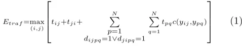
D. Objective: The cost functionEtraf representing the

maximum transmission time should be minimized:

Etraf=max

(i,j)

  tij+tji+

N ∑

p=1

dijpq=1∨djipq=1 N ∑

q=1

tpqc(yij,ypq)    (1)

where tij represents the traﬃc along the link from

APi→APj, andyij represents its assigned channel.

3 Proposal of SAP Allocation Algorithm

3.1 SAP Allocation Algorithm

Previously, we have proposed the routing tree algorithm and the NIC/channel assignment algorithm for WIMNET [4]. The former algorithm finds the communication route between the GW and the APs for a given AP network with the fixed SAPs. The latter algorithm finds the num-ber of NICs assigned to each SAP and the channel as-signment to each NIC for a given routing tree. Then,

because the cost function Etraf in the SAP allocation

problem can be calculated only after the routing tree and the NIC/channel assignment are found, our algorithm ap-plies these algorithms to any feasible SAP allocation for a given AP network, and selects the best one that

mini-mizesEtraf. Here, to reduce the computation time, our

algorithm discards undesirable SAP allocations by

adopt-ing the maximum estimated SAP load before applying

previous algorithms. The following procedure describes the details of the SAP allocation algorithm:

(1) Calculate the lower boundNSAP

LB on the number of

SAPs, which is equal to the number of WDS clusters.

If the input number of SAPsM is smaller, then set

M=NSAP LB =

⌈ _N

W SIZE

⌉

.

(2) Generate a new SAP allocation by selectingM APs

for SAPs amongN APs.

(3) Check the feasibility of the SAP allocation ofNSAP

LB

of satisfying the three constraints. If it is not feasi-ble, go to (8).

(4) Calculate the maximum estimated SAP load in

Sect. 3.2. If it is larger than the threshold there, go to (8).

(5) Apply the routing tree and NIC/channel assignment

algorithms in [4]. If no feasible solution is obtained, go to (8).

(6) Calculate the cost functionEtraf.

(7) Update the best-found solution if Etraf in (6) is

smaller than the best one.

(8) Terminate the procedure if every SAP allocation is

generated in (2). Otherwise, go to (2).

3.2 Maximum Estimated SAP Load

As the number of APs increases for a large-size WIM-NET, the number of SAP allocations increases exponen-tially. Then, the computation time becomes unaccept-ably long, where the routing tree and NIC/channel as-signment algorithms inhibitory requires the long time. To

avoid this situation, themaximum estimated SAP loadis

calculated for each SAP allocation before their applica-tions, and if the value is larger than the threshold, it is discarded because traﬃcs are concentrated into a speciﬁc SAP that may become the bottleneck of WIMNET.

3.2.1 SAP Selection Weight by Hop Count

As the WDS cluster head of a CAP, a SAP with the smaller hop count (number of hops) has the larger pos-sibility than a SAP with the larger hop count due to the

delay. Thus, theSAP selection weightby hop count is

cal-culated for each pair of a SAP and a CAP to represent

the possibility of being the same cluster by Wk= 1/2k.

3.2.2 Procedure for Maximum Estimated SAP

Load

For each SAP in a SAP allocation, the maximum

esti-mated SAP loadis calculated by the following procedure:

(1) Find the connectable SAPs for each CAP in the SAP

allocation.

(2) Calculate the weighted average of theSAP selection

weightsamong the connectable SAPs for each CAP.

(3) Multiply the maximum expected number of

associ-ated hostshi to this weighted average for each SAP.

(4) For each SAP, sum up the values ofWkinof all the

CAPs that can select this SAP as the cluster head,

which becomes theestimated SAP load.

(5) Select the maximum value of (4) among all the SAPs

in the SAP allocation for the maximum estimated

SAP load.

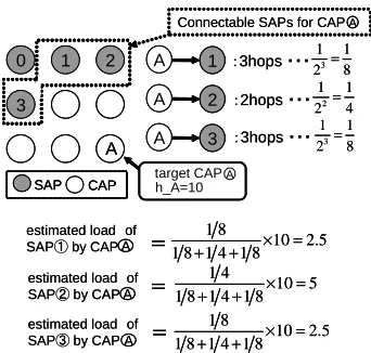
[image:3.595.53.292.172.218.2]

3.2.3 Example of Estimated SAP Load

Figure 2 illustrates an example of calculating the

(4)

are connectable for CAP-A. Because the hop count from CAP-A is three, two, and three to each SAP, the corre-spondingSAP selection weightsare given by: 1/23_{, 1}/₂2_, 1/23_{. Because}_h

ifor CAP-A is 10, the estimated load for

each of the three SAPs by CAP-A is 2.5, 5, and 2.5 as

shown in Fig. 2. Then, after calculating them for every

CAP, theestimated SAP load is calculated by summing

up them for each SAP.

0 1 2 A 1

3

A

A 2

A 3

：3hops ・・・

：2hops ・・・

：3hops ・・・

SAP CAP

Connectable SAPs for CAP

3 1 1 2 =8

2 1 1 2 =4

target CAP A

1 8

10 2.5 1 8 1 4 1 8+ + × =

＝ estimated load of

SAP①by CAP A

A

h_A=10

1 4

10 5 1 8 1 4 1 8+ + × =

＝

1 8

10 2.5 1 8 1 4 1 8+ + × =

＝ A

A estimated load of

SAP②by CAP

estimated load of

SAP③by CAP

0 1 2 AA 11

3

A

A 2

A 3

：3hops ・・・

：2hops ・・・

：3hops ・・・

SAP CAP

Connectable SAPs for CAP

3 1 1 2 =8

2 1 1 2 =4

target CAP A

1 8

10 2.5 1 8 1 4 1 8+ + × =

＝ estimated load of

SAP①by CAP A

A

h_A=10

1 4

10 5 1 8 1 4 1 8+ + × =

＝

1 8

10 2.5 1 8 1 4 1 8+ + × =

＝ A

A estimated load of

SAP②by CAP

estimated load of

SAP③by CAP

Figure 2: Example of estimated SAP load calculation.

3.2.4 Threshold for Traﬃc Concentration

Themaximum estimated SAP loadis compared with the

given thresholdT hto judge whether the SAP allocation

may cause the traﬃc concentration into a speciﬁc SAP or not. If it exceeds the threshold, the SAP allocation is discarded. For this threshold, the twice of the average SAP load is used:

T h=

(∑N i=1hi

M

)

×2. (2)

4 Evaluation by Simulations

In this section, we evaluate the proposed SAP alloca-tion algorithm in terms of the computaalloca-tion time and the throughput by packet transmission simulations us-ing the WIMNET simulator. For simulations, we prepare three AP network topologies with diﬀerent communica-tion loads. Each simulacommunica-tion assumes that at the begin-ning, every host posses 125 packets to the GW

(Inter-net) and the GW does 1,000 packets to every host. The

bandwidth is 30M bpsfor any link between two APs and

20M bpsfor that between an AP and a host. When mul-tiple links within interference ranges try to be activated simultaneously, randomly selected one link among them is successfully activated, and the others are inserted into

waiting queues. After every packet reached the destina-tion, the throughput is calculated by dividing the total packet size with the simulation time.

4.1 Simulated Instances

topology 1 adopts the gird one in Fig. 3 that has been

often used in mesh network studies. 25(= 5×5) APs are

allocated on the grid, where the center AP is selected as the GW. Each AP can communicate wirelessly with its four neighbor APs. As network loads, two diﬀerent traﬃc patterns are prepared, where the black circle represents

a crowded AP associating 8 hosts for pattern 1 and 10

hosts forpattern 2, and the white circle represents an AP

associating only 1 host, so that about 100 hosts totally

exist in each pattern. The WDS cluster size W SIZE is

set 8, which indicates that the lower bound on the number

of clustersNSAP

LB is 4 from

⌈₂₅ 8

⌉

= 4. Actually, we select

m= 5 because it gave the similar throughput to the case

where every AP is selected as a SAP in our preliminary experiments.

pattern1 pattern2

[image:4.595.83.254.181.344.2]

pattern1 pattern2

Figure 3: Network topology and traﬃc patterns for

topol-ogy 1.

topology 2 adopts the same gird topology as topology 1

with increasing 49 APs, to investigate the scalability of our algorithm. The number of crowded APs (black cir-cles) is also increased, and the number of SAPs is dou-bled.

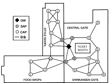
topology 3 in Fig. 4 adopts a topology that models the second floor at JR Okayama station, to consider the more practical field. The AP allocation and network loads are given by considering the floor structure and the flow of people there. We note that the number inside a circle represents the maximum expected number of hosts at the AP. The AP around the field center is selected as the GW where no host is associated.

4.2 Evaluation of Cost Function

First, we evaluate the validity of the cost function Etraf

in terms of the throughput obtained by the WIMNET simulator. For each simulation, we use the solution (the SAP allocation, the routing tree and NIC/channel as-signments) of our algorithm as the WIMNET

conﬁgura-tion. Here, the maximum number of NICs per SAP Q

is four fortopology 1andtopology 2and ﬁve fortopology

(5)

FOOD SHOPs link SAP

CAP GW

1

10 1 1

2 1 1

6 6

6

9 9

9

9 4

5

SHINKANSEN GATE CENTRAL GATE

S

T

Y

L

E

S

H

O

P

s

TICKET BOOTH

FOOD SHOPs link SAP

CAP GW

link SAP

CAP GW

1

10 1 1

2 1 1

6 6

6

9 9

9

9 4

5

SHINKANSEN GATE CENTRAL GATE

S

T

Y

L

E

S

H

O

P

s

[image:5.595.78.260.70.209.2]

TICKET BOOTH

Figure 4: Network topology and traﬃc patterns for

topol-ogy 3.

is 120M bpsfor the ﬁrst two topologies and 150M bpsfor

the last. Figures 5 and 6 show the relationship graph between the cost function and the throughput at each

traﬃc pattern fortopology 1, Figs. 7 and 8 do it for

topol-ogy 2, and Fig. 9 does it fortopology 3, respectively. In any graph, the throughput becomes maximum when the cost function is minimum, which supports the validity of our cost function.

0 20 40 60 80 100

0 100 200 300 400

cost function E_traf th

ro ug hp ut （M bp s）

Figure 5: Relationship between cost function and

[image:5.595.343.513.78.179.2]

throughput atpattern 1fortopology 1.

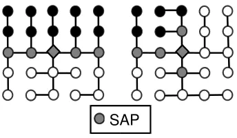
Figure 10 illustrates the SAP allocation and the routing

tree at each traﬃc pattern for topology 1 by our

algo-rithm. Any solution satisﬁes the constraints of the SAP allocation problem and balances the loads well between SAPs.

4.3 Evaluation of Maximum Estimated SAP

Load

Then, we evaluate the eﬀectiveness of the use of the

max-imum estimated SAP load in reducing the computation time of our algorithm.

First, we verify the validity of theSAP selection weight

by hop count. Table 1 shows the relationship between the hop count and the selected rate such that a certain SAP/CAP pair is actually included in the routing tree by

0 20 40 60 80 100

0 100 200 300 400 500 cost function E_traf

th ro ug hp ut （M bp s）

0 20 40 60 80 100

0 100 200 300 400 500

[image:5.595.343.513.256.365.2]

our algorithm. This table indicates that the selected rate

roughly becomes 1/2 every time the hop count increases

by one, which supports the validity of ourSAP selection

weight by hop count.

Then, to evaluate the eﬀectiveness of the maximum

es-timated SAP load in terms of the computation time re-duction, we count the number of SAP allocations where the routing tree and NIC/channel assignment algorithms are applied, when each of the three constrains ((1), (2), (3)) and the maximum estimated SAP load ((4)) is

se-quentially applied. Table 2 shows that fortopology 1and

topology 3 with a fewer numbers of APs and SAPs, the

maximum estimated SAP loadreduces it into about 2/5 of

the result by the constraints, and fortopology 3, it does in

[image:5.595.86.255.392.493.2]

about 1/6. Thus, the use of themaximum estimated SAP

Table 1: Relationship between hop count and SAP/CAP pair selected rate.

1 hop 2 hops 3 hops 4 hops

topol. 1, pat. 1 80.0% 38.4% 7.1% 0.0%

topol. 1, pat. 2 72.2% 33.3% 22.2% 8.3%

topol. 2, pat. 1 58.8% 30.7% 21.2% 8.3%

topol. 2, pat. 2 64.7% 31.5% 20.4% 9.6%

[image:5.595.308.548.682.757.2]

(6)

0 20 40 60 80 100

0 100 200 300 400 500 600 cost function E_traf

[image:6.595.342.514.71.171.2]

th ro ug hp ut （M bp s）

0 20 40 60 80 100

0 100 200 300 400

throughput fortopology 3.

loadis very eﬀective to reduce the computation time.

Table 3 shows the total computation time of our

algo-rithm on a PC withCore 2 Duo 2.67 GHzfor CPU,3.25

GBfor main memory, andLinux 2.6.16for OS. With the

help of themaximum estimated SAP load, our algorithm

can run within acceptable time for a large-scale WIM-NET.

5 Conclusion

This paper presented the deﬁnition of the smart access point (SAP) allocation problem for the scalable

wire-less Internet-access mesh network WIMNET and its

al-Table 2: Number of examined SAP allocations by algo-rithm.

(1) (1),(2) (1) -(3) (1)-(4)

topol. 1, pat. 1 251 243 243 147

topol. 1, pat. 2 251 243 243 107

topol. 2, pat. 1 173252 108544 33208 5384

topol. 2, pat. 2 173252 108544 33208 6513

topol. 3 229 203 203 164

Figure 10: SAP allocation and routing tree for topology

[image:6.595.86.254.78.181.2]

1.

Table 3: Algorithm computation time (seconds).

topol. 1 topol. 1 topol. 2 topol. 2 topol. 3 pat. 1 pat. 2 pat. 1 pat. 2

22 18 4692 4941 20

gorithm adopting the maximum estimated SAP loadfor

the computation time reduction. The effectiveness of our proposal was verified through simulations in three net-work topologies using the WIMNET simulator. Our fu-ture works may include extensions of the SAP allocation algorithm to dynamic changes of network loads and net-work configurations by failures of links or access points, and evaluations in the real network after the SAP imple-mentation.

References

[1] Akyildiz, I. F., Wang, X., Wang, W., ”Wireless mesh

networks: a survey,”Comput. Network, vol. 47, no.

4, pp. 445-487, March 2005.

[2] Farag, T., Funabiki, N., Nakanishi, T., ”An access point allocation algorithm for indoor environments

in wireless mesh networks”, IEICE Trans.

Com-mun., vol. E92-B, no. 3, pp. 784-739, March 2009.

[3] Hirakata, K., Horiuchi, T., Funabiki, N., Nakanishi, T., ”A construction of the smart access point for

practical wireless mesh networks,”IEICE Tech.

Re-port, vol. NS2008-99, pp. 63-68, Nov. 2008.

[4] Uemura, K., Funabiki, N., Nakanishi, T., ”A com-munication route optimization algorithm for scalable

wireless mesh networks,”IEICE Trans. B, vol.

J92-B, no. 9, Sep. 2009.

[5] Hsiao, P.-H., Hwang, A., Kung, H. T., Vlah, D., ”Load-balancing routing for wireless access

net-works,”Proc. IEEE INFOCOM, vol. 2, pp. 986-995,

April 2001.

[6] JR Okayama Station,

[image:6.595.85.255.257.355.2]