Flow and Heat Transfer In a Power-law Fluid
with Variable Conductivity over a Stretching
Sheet
Jing zhu
1, Liancun Zheng
1, Xinxin Zhang
2 ∗Abstract—The steady, laminar incompressible MHD stagnation-point flows and heat transfer with variable conductivity of a Non-Newtonian Fluid over a stretching sheets are analyzed for three cases of heating conditions, namely, (i)the sheet with the con-stant surface temperature; (ii) the sheet with the pre-scribed surface temperature; (iii) surface temperature with the prescribed surface heat flux. The governing system of partial differential equations is first trans-formed into a system of dimensionless ordinary dif-ferential equations. The numerical solutions are pre-sented to illustrate the influence of the various values of the ratio of free stream velocity and stretching ve-locity, the magnetic field parameter, Prandtl number, the wall temperature exponent and the power-law in-dex. These effects of the different parameters on the velocity and temperature as well as the skin friction and wall heat transfer are presented in tables and graphically. The results are found to be in good agre-ment with those of earlier investigations reported in existing scientific literatures.
Keywords: Non-Newtonian power-law fluid,
Stagna-tion point, Stretching sheet, Surface heat flux
1
Introduction
Flow of an incompressible viscous fluid and heat trans-fer phenomena over a stretching sheet have received great attention during the last decades owing to the abundance of practical applications in chemical and manufacturing processes, such as polymer extrusion, drawing of copper wires, continuous casting of metals, wire drawing and glass blowing. Since the pioneering work of Sakiadis[1], various aspects of the problem have been investigated by many authors. Crane[2] studied a steady flow past a stretching sheet and presented a closed form solution to it. Following them, Gupta[3] examined the heat and mass transfer using a similarity transformation for the boundary layer flow over a stretching sheet subject to suc-tion or blowing while Mahapatra and Gupta[4]studied the
∗1Department of Mathematics and Mechanics, University of
Sci-ence and Technology Beijing, Beijing 100083, China. e-mail: [email protected], [email protected] . 2 Mechanical
En-gineering School, University of Science and Technology Beijing. [email protected].
heat transfer in stagnation-point flow towards a stretch-ing sheet. Very recently, Layek et al.[5]investigated the stagnation-point flow of an incompressible viscous fluid towards a porous stretching surface embedded in a porous medium subject to suction/blowing with internal heat
generation or absorption. However, above researches
were restricted to flows of Newtonian fluids.
It’s worth mentions here that a number of industrially im-portant fluids such as molten plastics, polymers, pulps, foods and slurries exhibit Non-Newtonian fluid behav-ior. Because of the growing use of the Non-Newtonian fluid in various manufacturing and processing industries, the study of non-Newtonian liquid films are important. The theoretical analysis of an external boundary layer flow of a non-Newtonian fluid was first performed by Schowalter[6]. Zheng et al.[7] investigated the flow in a power-law fluid over a flat plate moving at constant speed in the direction and opposite to the direction of the main stream. The heat transfer aspect of such prob-lems had been considered recently by Chen[8]. Anders-son et al.[9] had further investigated the magnetohydro-dynamic flow over a stretching sheet of an electrically conducting incompressible fluid obeying the power-law model. Recently, Liao[10]–[11] obtained an accurate ana-lytic solution of unsteady magnetohydrodynamic flows of non-Newtonian fluids caused by an impulsively stretching plate.
field parameter, Prandtl number, the wall temperature exponent and the power-law index.
2
Flow analysis
Consider the steady MHD flow of a non-Newtonian power-law fluid near the stagnation point of a flat sheet coinciding with the plane y= 0, the flow being confined toy >0. xandy are the Cartesian coordinates with the origin at the stagnation point along and normal to the plate, respectively. Two equal and opposite forces are applied along the x-axis so that the local tangential ve-locity isuw=bx, wherebis a positive constant. It is also
assumed that the ambient fluid is moved with a velocity ue = cx, wherec > 0 is a constant. In this coordinate
system, the steady appropriate boundary-layer for two-dimensional MHD flow of a power-law fluid is described by the following equations
∂u ∂x+
∂v
∂y = 0, (1)
u∂u ∂x +v
∂u ∂y =ue
∂ue
∂x + 1 ρ
( ∂τxy
∂y )
+σB
2 0
ρ (ue−u), (2)
u(x,0) =bx, v(x,0) = 0, at y= 0, (3)
u(x,∞) =ue=cx, as y→ ∞. (4)
Whereuandv are the velocity components along thex -axes andy-axes, respectively. ρis the density of the fluid, andτxyis the shear stress. σis the electric conductivity,
B0 is the uniform magnetic field along the y-axis. The non-Newtonian fluid model used in this study is the power law model with the parameters defined by
τxy=k|
∂u ∂y|
n−1∂u
∂y. (5)
Where k is called consistency coefficient and υ =
k ρ|
∂u ∂y|
n−1is the kinematic viscosity. n is the power-law index. Near the sheet, we assume that the flow field is given by the stream function and similarity variabletas:
Ψ =xn2+1n f(t), t=x 1−n
1+ny, u=∂Ψ
∂y, v=− ∂Ψ
∂x. (6)
Further, introducing the following dimensionless quanti-ties and transformations
η=tb2n−+1n(nν0)
−1
n+1, g(η) =
n+1√ b1−2n
n+1√nν
0
f(t). (7)
Eq.(2) reduces to
|g00|n−1g000+ 2n n+ 1gg
00−(g0)2−M2(g0−c
b )
+ (c
b )2
= 0.
(8) The boundary conditions (3–4) may be expressed in di-mensionless form as
g(0) = 0, g0(0) = 1, g0(+∞) = c
b. (9)
Where M2 = σB02
bρ is the Hartman number, d =
c b is
velocity ratio parameter.
3
Heat transfer analysis
The energy equation for the above two-dimensional flow may be written
ρcp(u
∂T ∂x +v
∂T ∂y) =
∂ ∂y(λ(x)
∂T
∂y). (10)
Wherecpis the specific heat capacity andλ(x) is the
ther-mal conductivity which is assumed to be variable here.
3.1
Constant surface temperature
In this circumstance, the boundary conditions are
T(x,0) =Tw, T(x,∞) =T∞, (11)
whereTwis the wall temperature,T∞is the temperature
of the fluid far from the sheet.
Introducing the following dimensionless quantities
θ1=
T−T∞ Tw−T∞
. (12)
On using (6-7) and (12), the governing problem (10) is transformed to
λ(x)θ001x21+−2nnb
3−3n n+1n
−2
n+1ν
−2
n+1
0 +
2n n+ 1gθ
0
1= 0. (13)
If λ(x) = k0x
2n−2
1+n, Eq.(13) can be transformed to the
ordinary differential equation, wherek0 is constant. For conciseness, define the variable
λ(x) =λ0x
2n−2 1+nb
3n−3
n+1nn2+1ν 1−n n+1
0 ρcp,
Eq.(13) reduces to
θ001+P r 2n n+ 1gθ
0
1= 0, (14)
with boundary conditions
θ1(0) = 1, θ1(+∞) = 0, (15)
whereP r=ν0/λ0.
3.2
Prescribed surface temperature
Here, the boundary conditions are
T(x,0) =Tw=T∞+G(x), T(x,∞) =T∞. (16)
Where Tw is the wall temperature which is assumed to
be variable .
Introducing the following dimensionless quantities
θ2=
T−T∞ Tw−T∞
On using (6-7) and (17), Eq.(10) can be written
λ(x)G(x)θ200x21+−2nnb
4−2n n+1n
−2
n+1ν
−2
n+1
0 −bρcp
(
xg0θ2G0(x)−n2+1n gθ20G(x)
)
= 0. (18)
This equation cannot be transformed to the
or-dinary differential equation for arbitrary η unless
λ(x)G(x)x21+−2nn/xG0(x) = const, xG0(x)/G(x) =
const, λ(x)G(x)x21+−2nn/G(x) = const. Hence the
vari-able G(x) = Cxs and λ(x) = k
0x
2n−2
1+n, where the wall
temperature exponentsare constants.
For conciseness, define the variables
λ(x) =λ0x
2n−2 1+nb
n−2
n+1nn+12 ν 1−n
1+n
0 ρcp,
Eq.(18) reduces to
θ200+ 2n n+ 1P rgθ
0
2−sP rθ2g0= 0 (19)
with boundary conditions
θ2(0) = 1, θ2(+∞) = 0. (20)
3.3
Prescribed heat flow
In the PHF case, the boundary conditions are
qw=−λ(x)
∂T ∂y =Dx
m
, T(x,∞) =T∞. (21)
WhereD and the surface heat flux exponentmare con-stants,qwis the wall heat flux.
For the prescribed surface heat flux case, the dimension-less temperature is defined as
T−T∞=D P r ρcpn+1√nν0
n+1√
xm+1+mn−nθ
3(η). (22)
On using (6-7) and (22), Eq.(10) can be written
λ(x)θ003x21+−2nnb
4−2n n+1n−
2
n+1ν
−2
n+1
0 −bρcp
(
m−n+1+mn
1+n xg0θ3−
2n n+1gθ03
)
= 0 (23)
if λ(x) = k0x
2n−2
1+n, Eq.(23) can be transformed to the
ordinary differential equation, wherek0 is constant. For conciseness, define the variables
λ(x) =λ0x
2n−2 1+nb
n−2
n+1nn+12 ν 1−n
1+n
0 ρcp.
Eq.(30) and the boundary conditions of (21) are trans-formed to
θ300+ 2n n+ 1P rgθ
0
3−
m−n+ 1 +mn
1 +n P rθ3g
0= 0, (24)
[image:3.595.308.540.100.203.2]θ30(0) = 1, θ3(+∞) = 0. (25)
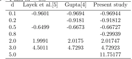
Table 1: Comparison off00(0) for several values ofdwith n= 1 and M = 0.0
d Layek et al.[5] Gupta[4] Present study
0.1 -0.9601 -0.9694 -0.96944
0.2 -0.9181 -0.91812
0.5 -0.6499 -0.6673 -0.66727
0.8 -0.29939
2.0 1.9991 2.0175 2.01747
3.0 4.5011 4.7293 4.72923
[image:3.595.279.546.235.372.2]5.0 11.75177
Table 2: Values off00(0) for several values ofd, nandM n M d= 0.1 d= 0.8 d= 1.5 d= 3.0
0.5 0.0 -0.72022 -0.15456 1.04129 6.22805
0.5 0.5 -0.83211 -0.16668 1.06949 6.42112
0.5 1.0 -1.13807 -0.20151 1.14846 7.00117
0.5 2.0 -2.09708 -0.31897 1.19967 9.10889
0.8 0.0 -0.88311 -0.24210 0.83329 5.21930
0.8 0.5 -0.98919 -0.25663 0.86846 5.34991
0.8 1.0 -1.26500 -0.29815 0.96791 5.72804
1.5 0.0 -1.11815 -0.43016 0.68395 3.87743
1.5 0.5 -1.19727 -0.44701 0.71989 3.94097
1.5 1.0 -1.39935 -0.49276 0.82776 4.12362
4
Results and discussion
The systems of ordinary differential equations
(8),(14),(19) and (24) with the aforementioned boundary conditions equations are solved numerically using means of the fourth–order Runge–Kutta method and shooting techniques until the free stream conditions are identically satisfied. In order to verify the accuracy of our present method, we have compared our results with those of Layek et al.[5] and Gupta[4]. The comparisons in all the above cases are found to be in good agreement, as shown in Table 1.
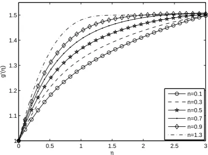
Figs.1-2 reveal the influence of the parameterd, non the horizontal velocity profiles g0(η) for flows of the Non-Newtonian fluids. Fig.1 shows the velocity profiles g0(η) for different values of the power-law indexnwithd= 1.5 and M = 0.5. It is observed that the velocity pro-files g0(η) change dramatically as n is varied. Fig.2 gives the effects of d on the velocity profiles g0(η) with M = 1.0, n = 0.5. It is noted that the variation of g0(η) depends on the ratio d = c/b of the velocity of the stretching surface to that of the frictionless potential flow in the neighborhood of the stagnation point and in-creases with increasing of parameter d= c/b. It is also observed that the flow has a boundary layer structure whenc/b >1 while an inverted boundary layer is formed forc/b <1. Further the thickness of the boundary layer decreases with increasing ofc/b.
P r, n and s, m on the dimensionless temperature dis-tributions θ1(η), θ2(η) and θ3(η). In the CST case we plot the dimensionless temperature profile θ1(η) with
M = 0.0, n = 0.5, d = 1.5, as shown in Fig.3 for the various values of P r. It can be clearly seen that the variation of θ1(η) decreases as P r increases. As antic-ipated, the thermal boundary layer thickness decreases with increasing Prandtl number. In the PST case we plot the dimensionless temperature profileθ2(η), as shown in Figs.4-5. It is noted that the variations of θ2(η) are de-creasing as s andn, respectively, increases. Fig.6 shows the fluid wall temperatureθ3(η)increases with increasing Prandtl number.
Finally, we compute the dimensionless shear stress at the wall and the wall heat flux. The computed variation of f00(0) with n, M and d has been summarized in Tables 2. It shows that the dimensionless shear stress f00(0) increases as d increases with all other parameter fixed. On the other hand, the variation of|f00(0)|increases with increasing the magnetic field parameter. Also, the wall temperature |θ20(0)| in PST case is increased as a result of the applied magnetic field as shown in Table.3. The effect of the power-law index is found to decrease both the dimensionless shear stressf00(0) and the wall temperature θ2(0) in CST case.
5
Conclusions
In this paper, we investigate the similarity solutions for the steady laminar incompressible MHD stagnation-point flows and heat transfer with variable conductivity of a Non–Newtonian Fluid subject to a transverse uniform magnetic field over a stretching sheets for three cases of heating conditions, namely, (i)the sheet with the constant surface temperature; (ii) the sheet with the prescribed surface temperature; (iii) surface temperature with the prescribed surface heat flux. The following observations have been made from the present analysis.
(1) The flows of Non-Newtonian fluids have a boundary layer structure whenc/b >1 while an inverted boundary layer is formed forc/b <1. As expected, boundary layer thickness decreases by increasingc/b.
(2) The horizontal velocity profileg0(η) increases with in-creasing of parameterd=c/b, n, M.
(3) The temperature profilesθ1(η) for the CST case and
θ2(η) for the PST case decrease asP rincreases. However, the temperature profilesθ3(η) for the PHF case increases with increasing Prandtl number.
[image:4.595.306.555.104.191.2](4) The variation ofθ2(η) is decreasing forP r, sandn. (5) The magnitude of the wall shear stressf00(0) increases as d increases. The variations of |f00(0)| and |θ20(0)| in CST case increase with increasing the magnetic field pa-rameter. The effect of the power-law index is found to decrease both the dimensionless shear stress f00(0) and the wall temperature θ02(0) for PST case. Also, the fluid
Table 3: Values of θ02(0) for several values ofP r, n and M withd= 1.5, s= 0.5
n M P r= 0.1 P r= 0.7 P r= 3.5 d= 6.7
0.5 0.0 -0.34209 -0.86511 -1.86734 -2.55372
0.5 0.5 -0.34274 -0.86567 -1.87056 -2.56021
0.5 1.0 -0.34579 -0.87337 -1.88359 -2.56892
1.5 0.0 -0.41073 -1.04001 -2.22557 -3.03578
1.5 0.5 -0.41097 -1.04107 -2.23129 -3.03985
1.5 1.0 -0.41157 -1.04473 -2.23821 -3.04842
wall temperatureθ03(0) increases with increasing Prandtl number in PHF case.
0 0.5 1 1.5 2 2.5 3
1 1.1 1.2 1.3 1.4 1.5
η
g’(
η
)
[image:4.595.320.528.256.410.2]n=0.1 n=0.3 n=0.5 n=0.7 n=0.9 n=1.3
Fig.1 Effect of power-law index for variation ofg0(η) withd= 1.5 andM= 0.5.
0 0.5 1 1.5 2 2.5 3 3.5 4 4.5 5
0 0.2 0.4 0.6 0.8 1 1.2 1.4 1.6 1.8 2
η
g’(
η
)
[image:4.595.324.529.461.608.2]d=2.0 d=1.5 d=1.2 d=0.5 d=0.3 d=0.1
Fig.2 Velocity profilesg0(η) of flow for different values ofdwith
M= 1.0 andn= 0.5.
References
[1] Sakiadis,B.C. Boundary-layer behavior on contin-uous solid surfaces: Boundary-layer equations for two-dimensional and axisymmetric flow,AIChE J.,7, pp.26–28 1961
[2] L.J. Crane. Flow past a stretching sheet.
0 1 2 3 4 5 0
0.1 0.2 0.3 0.4 0.5 0.6 0.7 0.8 0.9 1
η θ1
(
η
)
Pr=0.3 Pr=0.7 Pr=3.0 Pr=6.7
Fig.3 Effect of Prandtl number for variation ofθ1(η) with
M= 0.0 andn= 0.5,d= 1.5.
0 1 2 3 4 5
0 0.1 0.2 0.3 0.4 0.5 0.6 0.7 0.8 0.9 1
η
θ2
(
η
)
s=0.0 s=1.0 s=1.5 s=2.0
Fig.4 Effect of the wall temperature exponent for variation of
θ2(η) withM= 0.0, P r= 0.7 andn= 0.5,d= 1.5.
0 1 2 3 4 5
0 0.1 0.2 0.3 0.4 0.5 0.6 0.7 0.8 0.9 1
η θ2
(
η
)
n=0.1 n=0.5 n=1.1 n=2.0
Fig.5 Effect of power-law index for variation ofθ2(η) with
M= 0.5, P r= 0.7 ands= 0.5,d= 1.5.
0 0.5 1 1.5 2 2.5 3 3.5 4
−1 −0.8 −0.6 −0.4 −0.2 0
η
θ3
(
η
)
Pr=0.7 Pr=3.0 Pr=6.7
Fig.6 Effect of Prandtl number for variation ofθ3(η) with
M= 0.5,m= 0.5,d= 1.5, andn= 0.5.
[3] Gupta, P.S., Gupta.A.S., Heat and mass transfer on a stretching sheet with suction or blowing. Canad. J. Chem. Eng, 55 pp.744–746 1977
[4] Mahapatra,T.R., Gupta.A.S., Heat transfer in
stagnation-point flow towards a stretching sheet. Heat and Mass Transfer, 38 pp.517–521 2002
[5] Layek ,G.C., Mukhopadhyay,S., Samad, Sk. A., Heat and mass transfer analysis for boundary layer stagnation-point flow towards a heated porous stretching sheet with heat absorption/generation
and suction/blowing. Int. Commu. Heat mass
Transter, 34 pp.347–356 2007
[6] Schowalter,W.R., The application of boundary-layer theory to power-law pseudoplastic fluids:Similar so-lution.AIChE J.,6 pp.24–28 1960
[7] Zheng,L.C., Ma, L., He, J., Bifurcation solution to a boundary layer problems arising in theory of power law fluids.Acta Math.Sci, 20 pp.19–26 2000
[8] Chen, C.H., Heat transfer in a power-law fluid film over a unsteady stretcgibg sheet.Heat Mass Trans-fer, 39 pp. 791–796 2003
[9] Andersson,H.I., Holmedal,B., Dandapat,B.S.,
Gupta.A.S., Magnetohydrodynamic melting flow
from a horizontal rotating disk. Math. Models
Methods Appl. Sci, 3 pp.373–393 1993
[10] Xu,H., Liao.S.J., Series solutions of unsteady mag-netohydrodynamic flows of non–Newtonian fluids caused by an impulsively stretching plate. J, Non– Newtonian Fluid Mech, 129 pp.46–55 2005